Burn Math Class: And Reinvent Mathematics for Yourself (2016)

2. The Infinite Power of the Infinite Magnifying Glass

2.3. Understanding the Magnifying Glass

In this section we’ll try to get better at using our infinite magnifying glass. Even though we invented it ourselves, it’s not entirely clear what we invented or how it behaves. That is, even though we invented the idea, we haven’t had a lot of practice actually using it on specific machines. In this section we’ll get a lot of practice by playing with a bunch of different examples. The only machines we know about are ones that can be completely described in terms of addition and multiplication, so that’s the only kind of machine we’ll play with at this point.

2.3.1Back to the Times Self Machine

Okay, so we’ve tested our infinite magnifying glass idea on machines that look like M(x) ≡ #, and we got M′(x) = 0. We tested it on different machines that look like M(x) ≡ ax + b, and we got M′(x) = a. Up to that point, we had only rediscovered things that we could have discovered with the normal slope formula and no infinite zooming in.

Then we tested our infinite magnifying glass on our first curvy thing: the machine M(x) ≡ x², and we got M′(x) = 2x. Before we move on to any different examples, let’s make sure we understand what this is saying by looking at it in two different ways.

2.3.2The Usual Interpretation: The Machine’s Graph Is Curvy

The first way of looking at this is the usual way: “graphing” M(x) ≡ x² and seeing that the graph is curvy. This is what we’re doing in Figure 2.3.

We imagine laying a bunch of Times Self Machines next to each other along the horizontal axis. We feed them the numbers on the horizontal axis, and what they spit out we draw on the vertical axis. The machine next to the number 3 is fed x = 3, and it spits out M(x) = 9, which is why we drew the height of the curvy thing at x = 3 to be 9. All the other places on the graph say essentially the same thing.

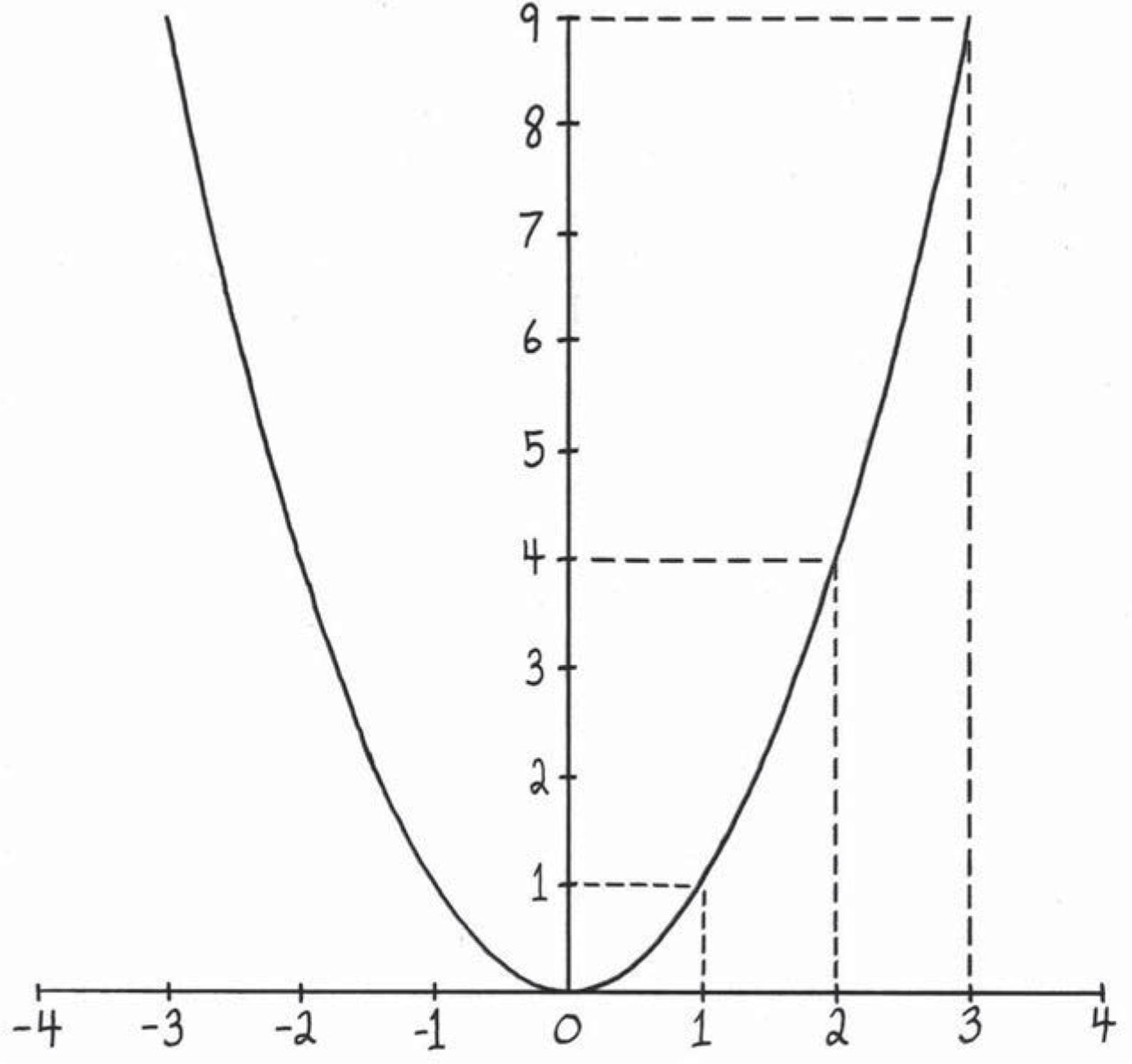
Figure 2.3: Visualizing the Times Self Machine M(x) ≡ x². The numbers in the horizontal direction are different things we can feed it, and the numbers in the vertical direction (the height) tell us what it spits out. Since the graph is curvy, it has different amounts of steepness at different places, so while the sentence M(x) ≡ x² tells you the height at x, the sentence M′(x) = 2x tells us the steepness atx. The graph is flat in the middle (at x = 0), so the steepness should be zero there. Fortunately, M′(x) tells us this too, because M′(0) = 2 · 0 = 0.

So we chose a random point with horizontal position x and vertical position M(x). Then we zoomed in infinitely far on the curve at this point and found its steepness there using the simple old “rise over run” business that we invented in Chapter 1. When all the dust settled, we found that the steepness there was M′(x) = 2x. Since we chose to be agnostic about which particular number x was, we really did infinitely many calculations at once. So the sentence M′(x) = 2x, in just a few symbols, manages to express an infinite number of sentences. Let’s see what some of them say.

One of these sentences says M′(0) = 2 · 0 = 0. This tells us that the steepness of the curve is zero when x = 0. If we look at Figure 2.3, this makes more sense. The graph is flat and horizontal there, so the steepness is zero. What about some of the other sentences hiding inside the infinite sentence M′(x) = 2x? Well, some other ones are:

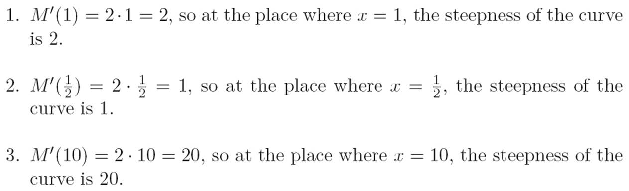
We could keep going, but all the sentences are saying basically the same thing. At a location with horizontal position h, the steepness of this curve is exactly 2h. So the steepness is always twice the horizontal distance away from 0. Just from this last sentence, we can see why the graph of M has to keep going up faster and faster. As the horizontal distance from zero gets bigger, the steepness is steadily increasing at every step.

2.3.3The Reinterpretation Dance: The Machine Has Nothing to Do with Curviness

Okay, so in the previous section we talked about the usual interpretation of the sentence “The machine M(x) ≡ x² has derivative M′(x) = 2x.” This interpretation involved graphing the machine M, noticing that it had different steepnesses in different places, and interpreting the derivative as telling us what the steepness was at different points.

But I also promised that we’d be able to look at it a second way, so let’s do that now. We’ll arrive at all the same conclusions by thinking about this machine differently. To start, notice that we don’t have to visualize the Times Self Machine by graphing it. We can also visualize it by thinking ofM(x) ≡ x² as the area of a square whose length on each side is x. Since we’re thinking about it differently now, let’s use the abbreviation A instead of M, and ℓ instead of x. Then we can write A(ℓ) ≡ ℓ², and we’d still be talking about the exact same machine, but we’re not thinking of it as talking about anything curvy now.

As always in calculus, we’ve got a machine, and we’re asking a question like, “If I change the stuff I’m feeding it by a tiny amount, how does the machine’s response change?” Since d is the first letter of “difference” and ℓ is the first letter of “length,” let’s use the abbreviation dℓ to stand for some tiny difference in length. We’re thinking of dℓ as a change we’re making to the side length of a square, so ℓ_after ≡ ℓ_before + dℓ. When we change the length a little bit, we can ask how the area changed. The area before the change is ℓ², and the area after the change is (ℓ + dℓ)². Let’s write all this in a box.

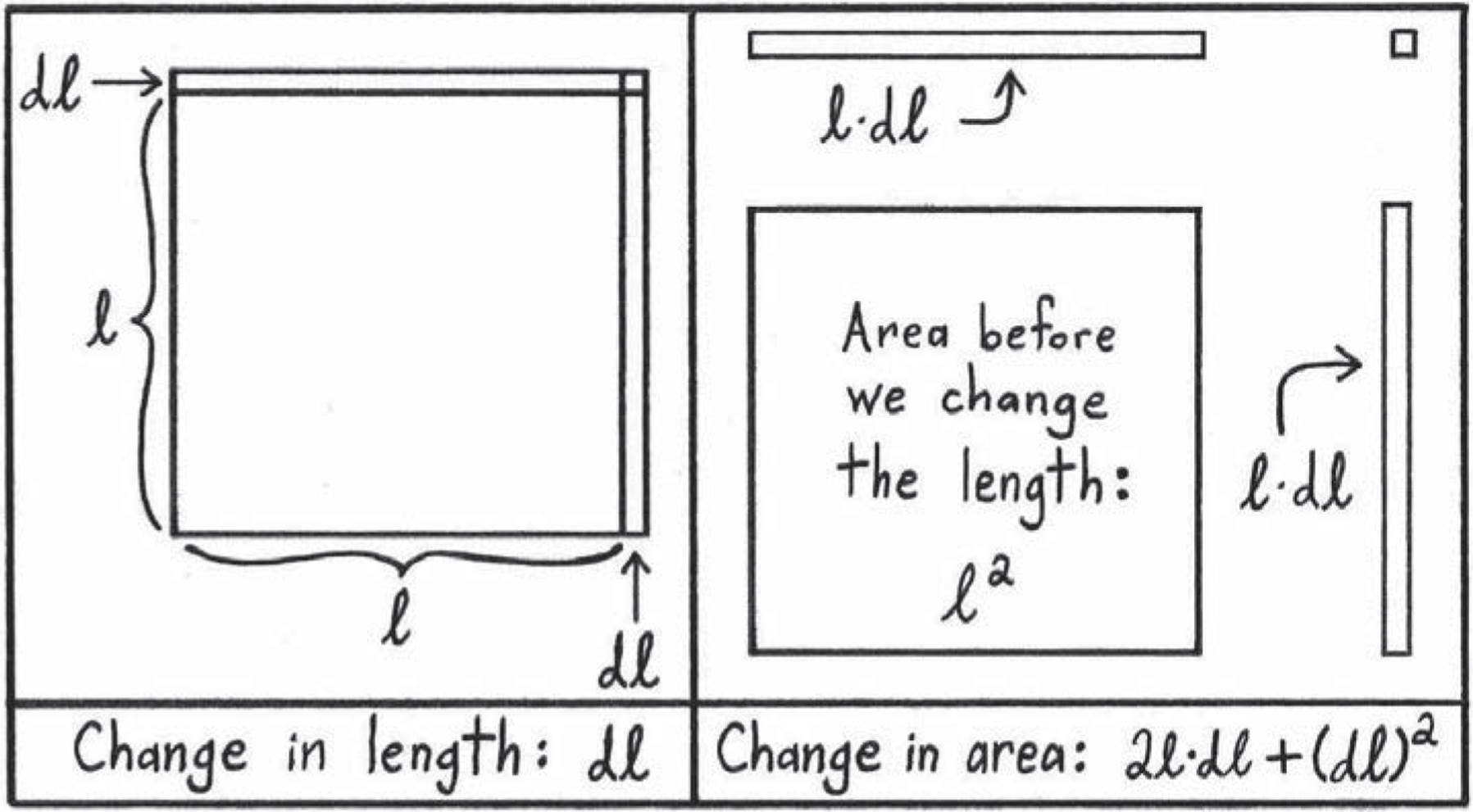
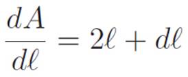
Figure 2.4: Another way of understanding the derivative of the Times Self Machine A(ℓ) ≡ ℓ². Originally, we have a square that is ℓ long on all sides. Then we change ℓ a tiny bit to make it ℓ + dℓ. Then we see how the area changed. From the picture, the change in area will be dA ≡ A_after − A_before = 2(ℓ · dℓ) + (dℓ)². So before shrinking dℓ down to zero, we have . Then shrinking dℓ down to zero (or if you prefer, thinking of it as “infinitely small” from the beginning), we get that the derivative is . We can think of the sentence as saying that the two long thin rectangles shrink to two lines (hence the 2ℓ), while the tiny square shrinks down to a point (hence the dℓ), which only adds an infinitely small length to either of those lines, so we can ignore it and just write .

Making Tiny Changes to a Square:

Length before we change it: ℓ

Length after we change it: ℓ + dℓ

Change in length: dℓ = ℓ_after − ℓ_before

Area before we change it: ℓ²

Area after we change it: (ℓ + dℓ)²

Change in area: dA = A_after − A_before

So we changed what we’re feeding the machine by a tiny amount. How does the stuff it spits out change? Let’s draw a picture. Our picture is in Figure 2.4, and it shows how the area changes when we change the side lengths a little bit. Here are different ways we could abbreviate the resulting change in area:

dA ≡ A_after − A_before ≡ A(ℓ + dl) − A(ℓ)

The picture makes it clear that this change in area will be

dA = 2(ℓ · dℓ) + (dl)²

This is just another way of saying

Then, shrinking dℓ down to zero (or if you prefer, thinking of it as infinitely small from the beginning, so that 2ℓ + dℓ will be indistinguishable from 2ℓ), we find that the “derivative” of the Times Self Machine A(ℓ) ≡ ℓ² is

This is the same sentence we found earlier, when it was written as M′(x) = 2x. In both cases, it was saying that the “derivative” or “steepness” or “rate of change” of the Times Self Machine at any number we feed it is two times as big as the number itself.

2.3.4What We’ve Done So Far

We’re still only thinking about machines that can be completely described using addition and multiplication. So we still don’t know anything about any of those bizarre machines you might have heard of, like sin(x), ln(x), cos(x), or e^x. We still have no idea what the area of a circle is, we don’t know what π means, and so on. We basically don’t know much except addition, multiplication, the idea of a machine, how to invent a mathematical concept, and a bit of calculus. The first mathematical concepts we invented were “area,” in the easy case of rectangles, and “steepness,” in the easy case of straight lines. Then we noticed that curvy stuff turns into straight stuff if you zoom in infinitely far, so we invented the idea of an infinite magnifying glass. This lets us talk about the steepness of any machine M whose graph is curvy, just by finding the “rise over run” of two points that are infinitely close to each other, like this:

Even though we feel like this idea should work for any machine we can describe at this point, we still haven’t played around with our infinite magnifying glass much yet. So far, we’ve only used it on constant machines, lines, and the Times Self Machine. Of these, only the last one was curvy, so we’ve really only played with the full power of our infinite magnifying glass in one example. Let’s play some more to try to get used to it.

2.3.5On to Crazier Machines

The Machine M(x) ≡ x³

If we want to play around with our infinite magnifying glass some more, we’ve got to think of some machines to use it on. Let’s try M(x) ≡ x³. So far, we’ve used the two abbreviations tiny and dx to stand for a tiny (possibly infinitely small) number. We also used dℓ, but that’s the same type of abbreviation as dx. We could use either of those, but both of them are fairly clunky. Let’s use the one-letter abbreviation t to stand for tiny. Just like before, t is a tiny (possibly infinitely small) number. So we want to feed the machine x, and then feed it x + t, and see how its response changes. Let’s use dM as an abbreviation for the change in its response, or dM ≡ M(x + t) − M(x). Then

The (x + t)³ piece will have a x³ hiding inside it, so that’s going to kill the negative x³ on the right side of dM, but we can’t see what the leftovers will look like unless we do the tedious job of breaking (x + t)³ apart. (Soon we’ll discover a way to avoid this.)

This is a pretty ugly sentence, and no one would want to memorize it. Fortunately, we saw how to invent the above sentence in Chapter 1, either by drawing a picture and staring at it, or by using the obvious law of tearing things a few times. As ugly as it is, equation 2.2 gives us another way of writing equation 2.1. That is:

where the numbers above the equals signs tell you which equation to look back to if you aren’t sure what we did. Everything has at least one t attached to it, so if we divide by that, we get

Notice that 3x² is the only piece that doesn’t have any t’s still attached. But remember that t was our abbreviation for an infinitely tiny number, or if you prefer, a number that we can imagine making smaller and smaller until we don’t notice it anymore. So we can rewrite this as

The term GonnaDie(t) is an abbreviation for all the stuff that’s gonna die when we turn the tiny number t all the way down to zero, and the piece on the far left is just the “rise over run” between two extremely close points, so it will turn into the derivative of M when we turn t down to zero. Let’s do that. Shrinking t down to zero gives

M′(x) = 3x²

Did it work? Well, we don’t know yet. We’re on our own here. Let’s keep moving, and maybe we’ll eventually figure out whether what we just did makes sense. (Don’t worry. It does.)

The Machines M(x) ≡ xⁿ

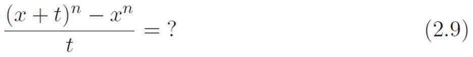
The hardest part of the example above wasn’t the calculus — that just involved throwing away all the pieces with a t attached. The hardest part was the tedious business of expanding (x + t)³. Let’s see if we can find the derivative of (i.e., use our infinite magnifying glass on) the machine M(x) ≡ x⁴without having to expand everything. Just like before, we want to calculate this:

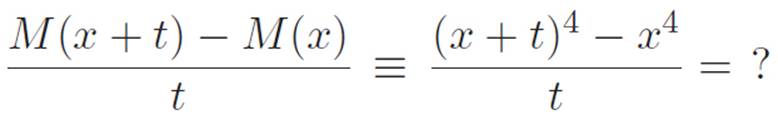
where t is some tiny number. We need to figure out a way to get rid of the t on the bottom⁵ so that we can just go ahead and turn t down to zero.

Why do we need to figure out a way to get rid of the t on the bottom? Because (tiny/tiny) isn’t really a tiny number! Similarly, if (stuff) is some normal number, not assumed to be infinitely small, then (stuff)(tiny)/(tiny) isn’t infinitely small either. It’s just equal to (stuff). So the reason we need to get rid of the t on the bottom is because it prevents us from seeing which pieces are really infinitely tiny, and which are normal numbers like 2 or 78.

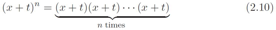
How can we avoid having to expand (x + t)⁴? Why avoid it at all? Well, expanding it all out wouldn’t be a very intelligent process. We’d waste a lot of time, and more importantly, we wouldn’t learn anything that would actually help us if we ever had to deal with (x + t)⁹⁹⁹, or (x + t)ⁿ. So let’s avoid expanding it, but still try to learn, in a vague sense, what the expanded answer looks like. The term we want to avoid expanding is (x + t)⁴, which is an abbreviation for

(x + t)(x + t)(x + t)(x + t)

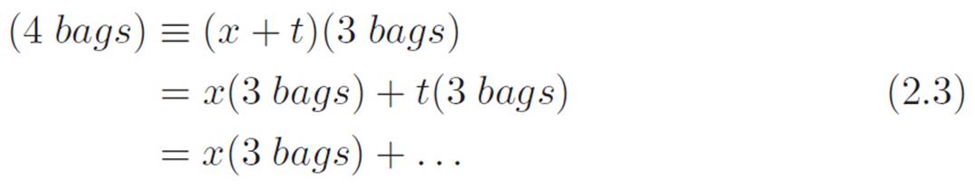
This can be thought of as four bags, each of which has two things inside it: an x and a t. If we took the time to expand all this nonsense, we’d get a result that was a bunch of pieces added together. We don’t care about the full expanded result. We just want to get a feel for what the individual pieces of the result would look like, so we can get a vague idea of how the final result might look without having to actually expand it all out. Suppose we use an abbreviation like this:

(x + t)(x + t)(x + t)(x + t) ≡ (4 bags) ≡ (x + t)(3 bags)

Imagine applying the obvious law of tearing things to the far right side, and then focusing in on one of the two pieces. Like this:

In the three lines above, we essentially tore open one bag, got two pieces out, and then picked one to focus on. Remember, we don’t care about every single term. We just want to see what an arbitrary piece in the end result looks like, to get an intuitive feel for how the end result is built. So since our goal is pretty modest, we can just keep ignoring all but one piece, like we did above, and keep on tearing the bags apart. Which side should we choose to focus on each time we tear? It doesn’t matter. Let’s just choose randomly. We just picked the x from the first bag, so let’s pick the t from the second, the t from the third, and the x from the fourth: x, t, t, x. Each time we unwrap, tear, and pick one term, I’ll write which one we picked above the equals sign. Each line below will be an abbreviation for three lines of reasoning just like those in equation 2.3: unwrap, tear, and focus. If that seems complicated, here’s all I mean:

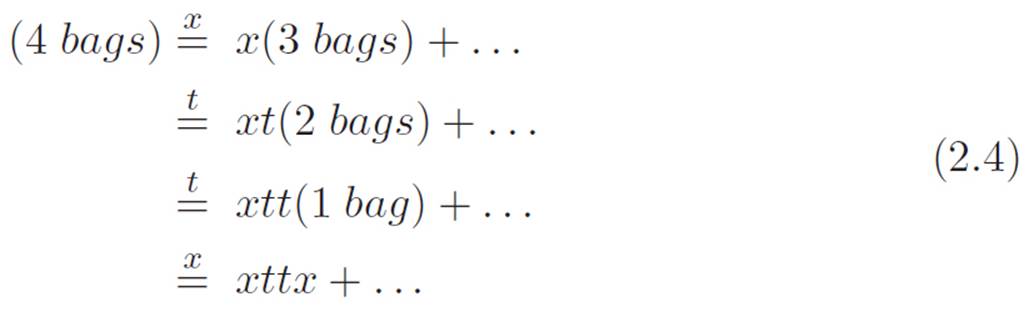
That wasn’t much work, but it turns out to give us exactly the information we wanted. We still don’t know what the full “expanded” result is, but we can now see that each term in the fully expanded version will be built from a choice. Or rather, four choices: a choice of one item from each bag. We just made our choice of xttx at random, so each other choice we could have made has to be in the final result as well. So without even expanding (x + t)⁴, we know that the fully expanded version will have an xttx, but there will also be an xxxx, and a tttt, and a xttt, and so on.

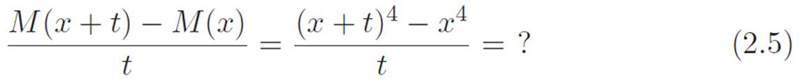
That’s really all we need to know. This simple knowledge makes it incredibly easier to compute the derivative of x⁴, or even xⁿ for that matter. Let’s return to the problem with this new bit of knowledge. We want to compute this:

Here’s the thought process:

1.One of the pieces in (x + t)⁴ will be xxxx, which is x⁴, but that gets killed by the negative x⁴ in the equation above (equation 2.5).

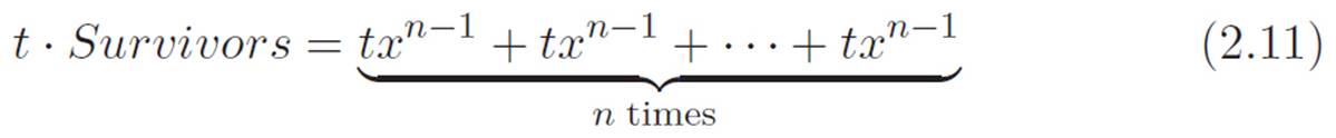
2.Some of the pieces in (x + t)⁴ will have only one t attached. That single t has to come from one of the four bags, so there should be four pieces with only a single t. That is, txxx, xtxx, xxtx, and xxxt. The single t in each will get killed by the t on the bottom of equation 2.5, turning each of those four terms into xxx, which is x³. That’s four copies of x³, or 4x³. Now, since these pieces won’t have any more t’s attached once we’ve canceled the t on the bottom, they won’t die when we turn all the t’s down to zero. Let’s write all of these pieces as t · Survivors to emphasize that they all only have one t hanging on to them, so when we divide them by t, they turn into Survivors, where Survivors is a bunch of stuff that doesn’t have any t attached. In this case, Survivors is just 4x³, but writing it in this more general way will help us make the argument for powers other than 4.

3.The rest of the terms will have more than one t attached, like ttxx or txxt. The t on the bottom of equation 2.5 will kill one of these, but they’ll all have at least one t still attached in the end, so these pieces will all die when we turn the t knob down to zero. Let’s call all these pieces t ·GonnaDie(t) to emphasize that they still have t’s hanging on even after we divide them by t, thus turning them into GonnaDie(t).

So, thinking about the problem this way, we can rewrite equation 2.5 using all the abbreviations we just decided on. Then we get:

The x⁴ pieces kill each other, and we can cancel the t’s to get

Now let’s imagine turning t down closer and closer to zero. This does nothing to the Survivors piece, but it kills GonnaDie(t). The left side turns into the derivative of M, which we’ll write as M′(x). Summarizing all that, we’ve got

Hey! So the derivative of M is just that term we called Survivors, which in this case was 4x³. But in that whole argument, starting at equation 2.5, we didn’t really use the fact that the power was 4. At least not in any important sense. So the same type of argument should work for the more general version (x + t)ⁿ, no matter what number n is.

The benefit of making the strange argument we just made — looking for general patterns, since we were too lazy to expand (x + t)⁴ in the usual tedious way — is that it instantly lets us figure out the derivative of xⁿ, no matter what number n is! Here’s how. To figure out the derivative of xⁿwhile remaining agnostic about n, we need to compute:

Now, just like before, let’s think in terms of bags. This time we have n of them:

Each piece of (x+t)ⁿ will be n things multiplied together, with various numbers of x’s and t’s. For example, one piece will be the guy with only x’s, or

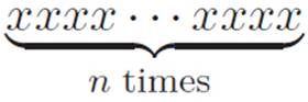
That’s xⁿ, and it gets canceled by the negative xⁿ in equation 2.9. Another one of the pieces will be the guy with a t in his second slot, a t in his final slot, and all the rest x’s, like this:

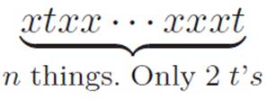
But this term has two t’s, so even after we cancel one of them against the t on the bottom of equation 2.9, there’s still at least one t left, so this term will die when we turn t down to zero, as will all the others with two or more t’s.

So we don’t have to expand (x + t)ⁿ using some complicated formula.⁶ As before, the derivative will only be affected by all the pieces with a single t, since those are the ones that will survive when their single t gets canceled by the t on the bottom of equation 2.9. One such piece will be txxx · · · xxxx, another one will be xtxx · · · xxxx, and so on. But each of these is just txⁿ−¹. There are n bags that a single t could come from, so the same term is just showing up n times.

The complicated formula textbooks use is called the “binomial theorem.” It’s basically a complicated way of talking about bags, like we did, but without saying that that’s what we’re doing, all while using a strange notation that looks almost like a fraction, but not quite. We can definitely do without it.

We can rewrite the same thing this way:

Since there’s one t on both sides, we can kill it off to get

But for the same reason as before, Survivors turns out to be the derivative of the machine we started with, which was M(x) ≡ xⁿ, so we can summarize this entire section by saying

What We Just Invented

If M(x) ≡ xⁿ,

then M′(x) = nxⁿ⁻¹

Now, you might trust the n = 2 calculation and the n = 3 calculation more than that crazy business about Survivors that we just did in this section, but notice that we can use our old results to check our new ones! If we were right that the derivative of machines like M(x) ≡ xⁿ is really M′(x) = nxⁿ−¹no matter what number n is, then this formula has to reproduce our old results, or else it’s wrong. That is, our new formula has to predict⁷ that the derivative of x² is 2x, and that the derivative of x³ is 3x². In fact, it does! When n = 2, the expression nxⁿ⁻¹ turns into 2x, and when n = 3, it turns into 3x². Now, you could still argue, “We shouldn’t feel completely certain that the above argument worked just because it gave us the right answers in the two cases where we knew what to expect!” You’d be right, but it does (and should) give us more confidence that we’re on the right track, and that we didn’t make any slip-ups in reasoning. In this process of inventing mathematics, it’s always up to us to decide when we’re convinced, since our mathematical universe doesn’t come pre-filled with books where we can simply look up the answer.

Or rather, “postdict”. . . Or maybe “retrodict”. . . Or something like that.

2.3.6Describing All of Our Machines at Once: Ultra-agnostic Abbreviations

Having played with our infinite magnifying glass by testing it on a bunch of specific machines, where do we go next? At the moment, the only machines we know about are ones that we can completely describe in terms of addition and multiplication. We’ve said the previous sentence so many times that it’s worth asking ourselves exactly what we mean. What kinds of machines can be “completely described” just “in terms of” addition and multiplication, that is, in terms of what we know? Well, of course it depends what we mean by that. For example, do we allow division in the description? It might seem like the answer should be no, because division doesn’t really exist in our universe. But it sort of does. The number in our universe is just an abbreviation for whichever number turns into 1 when we multiply it by s. But then what does it mean to describe something only in terms of addition and multiplication?

This is really just an issue of how we use words, so let’s not worry too much about it for now. We won’t allow “division” in the description, at least not yet, which just means we’re excluding machines like for the moment. What sorts of machines can we describe? Here are some:

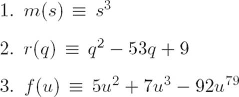
We don’t really have any reason to be interested in any of these machines, but we like our infinite magnifying glass, and we’d like to get better at using it. As we list more and more machines that can be described in terms of addition and multiplication, it starts to seem like there’s a pattern. All the machines we can describe at this point have a common structure. They’re all made out of pieces that look like this:

(Number) · (food)^number

where “food” is whatever abbreviation we’re using for what the machine eats (what textbooks call a “variable”) and where number isn’t necessarily the same as Number. All of the machines we listed above, and essentially any machine that we can completely describe in terms of what we know, is going to be a bunch of things that look like this, all added together. Why not “added and multiplied” together? Good question! That’s because two things that look like (Number)·(food)^number, when multiplied together, will be of the same form. That is, multiplying together something like axⁿ andbx^m gives (ab)x^n+m, which is just (Number) · (food)^number again. Okay, so any machine that we can completely describe in terms of addition and multiplication will be built from adding up pieces that look like this. Let’s come up with some abbreviations so that we can talk about any and all of our machines at once.

We need different abbreviations for a lot of different numbers. We only know what (stuff)^# means when # is a positive whole number,⁸ so in our universe, there’s no such thing as a negative or fractional power (yet!). So, since we’re only thinking about whole number powers at this point, we can write all of our machines like this:

Remember (stuff)^# is just an abbreviation for (stuff)(stuff) · · · (stuff), where the # is the number of times stuff shows up. If we’re being consistent about this, then (stuff)¹ should just be another way of writing (stuff).

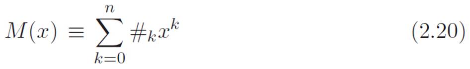
where n is the biggest power that shows up in the description of that particular machine, and the symbols #₀, #₁, #₂, . . ., #_n are just abbreviations for whatever numbers show up out front. We put subscripts on them so that we can tell them apart, and so we don’t have to use a different letter for each one. Also, we started the subscripts at 0 instead of 1 to make the rest of the subscripts match up with the powers, so that each piece (except the first one) looks like #_kx^k instead of #_kx^k−1. The only reason we did this was because it’s slightly prettier. If we just use x⁰ as an abbreviation for the number 1, then every single piece, including the first one, will look like #_kx^k. (There’s actually a better reason than this for choosing x⁰ = 1. We’ll see what that is in the next interlude.) At present, our choice to write x⁰ as an abbreviation for the number 1 is entirely a matter of aesthetics, and we’ll only use it so that every piece in equation 2.14 can be written to look like #_kx^k. For the moment, we have no reason to suspect that zero powers really are equal to 1 in any principled sense. We’re just abbreviating.

Okay, so equation 2.14 is an abbreviation that describes all of the machines that we can talk about at this point. Now, it’s fairly tedious to keep writing all the dots (these things → · · ·) in our description of these machines. So let’s invent a shorter way of saying the same thing. As an abbreviation for the right side of equation 2.14, we could write something like

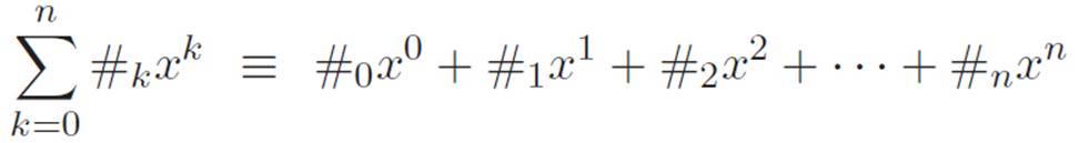
but this is a bit clunky too. We don’t need all those words on the right. We just need to remind ourselves where k starts and where it ends. So we could abbreviate the same thing this way:

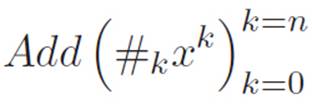
The way this is usually written in textbooks is

Actually, they usually use a letter like c (c stands for “constant”) instead of our number symbol #. They use a Σ (the Greek letter S) because S is the first letter of “sum,” and “sum” means “add.” This way of writing things can look scary before you’re used to it, but it’s just an abbreviation for the right side of equation 2.14, where we express the same thing using the “· · ·” notation. If you don’t like sentences with Σ, you can always just rewrite them by using the dots.

So we’ve built an abbreviation with enough agnosticism in it to let us talk about all of our machines at once. Since we’ve come up with a way of abbreviating them all, let’s come up with a name for them all too, so we don’t have to keep saying “machines that can be completely described using only addition and multiplication.” Let’s call any machine of the above form a “plus-times machine.” Based on everything we’ve talked about so far, you might have guessed that textbooks have some unnecessarily fancy name for this simple type of machine. In fact, they do! They call them “polynomials,” which isn’t the best term.⁹

Granted, the term “plus-times machine” isn’t the best either. It’s a bit awkward and clunky. But at least it reminds us what we’re talking about.

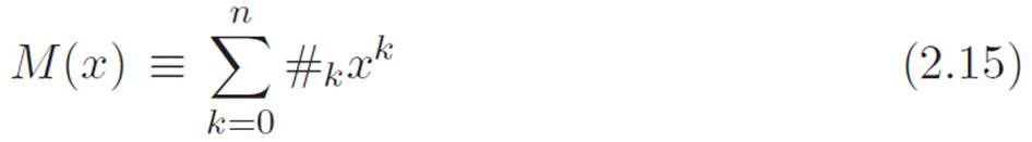
Anyways, if we could figure out how to use our infinite magnifying glass on any plus-times machine, then we would have truly progressed to a new level of skill in using it. Let’s try that, but first let’s summarize the above discussion, and make it official by writing it in its own box.

An Ultra-Agnostic Abbreviation

The strange symbols on the left are just an abbreviation for the stuff on the right:

Why: We’re using this abbreviation because we want to be able to talk about any machine that can be completely described using what we know: addition and multiplication.

P.S. The number symbols (i.e., #₀, #₁, #₂, . . ., #_n) are just normal numbers like 7 or 52 or 3/2. Writing symbols like # (instead of specific numbers like 7) lets us remain agnostic about which specific numbers they are. This way, we can secretly talk about infinitely many machines at once.

Name: We’ll call machines that can be written like this “plus-times machines.” Textbooks outside our universe usually call them “polynomials.”

2.3.7Breaking Up the Hard Problem into Easy Pieces

At this point, we only have two ways of figuring out the derivative of a machine. The first way is just to use the definition of the derivative — that is, to apply our definition of slope from Chapter 1 to two points that are infinitely close to each other. So if someone hands us a machine M, we can try to find its derivative by using this:

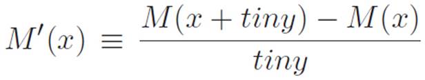
where tiny stands for some infinitely small number (or if you prefer, some tiny number, not necessarily infinitely small, which we imagine turning all the way down to zero after we’ve gotten rid of the tiny on the bottom).

The only other way we have of figuring out the derivative of a machine is to ask ourselves, “Have we figured out its derivative yet?” For example, we’ve figured out that the derivative of any machine that looks like M(x) ≡ xⁿ is just M′(x) = nxⁿ⁻¹, where n is any whole number. We could call this the “power rule,” like textbooks do, but of course that’s just a name for something we figured out ourselves, using the definition of the derivative. So I guess we really only have one way of figuring out the derivatives of things: the definition. As in all areas of mathematics, these “rules” (like the “power rule” textbooks talk about) aren’t really rules after all. They’re just names for things we figured out earlier. . . using the definition. . . The definition of a concept we created ourselves. . . starting from a vague, qualitative, everyday concept and falling back on aesthetics and anarchic whim whenever we didn’t quite know what to do. Huh. . . mathematics is weird. . .

Anyways, so we’ve written down an abbreviation that is large enough and agnostic enough to describe any machine in our universe. As a test of how far our skills have progressed in mastering the art of the infinite magnifying glass, let’s see if we can use it on any plus-times machine. Unfortunately, even though we managed to capture all our machines in a single abbreviation, it’s a pretty hairy one. If we just plugged the expression

into the definition of the derivative, we’d get a big ugly mess, and we probably wouldn’t know what to do. So let’s try to break apart this hard question into several easy questions that we can answer more easily.

Well, we’ve already made a helpful observation: any plus-times machine is just a bunch of simpler things added together. Our abbreviation in equation 2.15 says that these simpler things each look like #_kx^k, where k is some whole number, and #_k is any number, not necessarily a whole number. Maybe if we could figure out how to differentiate any machine that looks like #xⁿ, and if we could think of a way to talk about the derivative of a bunch of things added together in terms of the derivatives of the individual things, then we would have discovered a way to use our infinite magnifying glass on any plus-times machine. At that point, there would be no corner of our universe that we hadn’t conquered.

The Pieces: #xⁿ

We already figured out how to use our infinite magnifying glass on xⁿ. Its derivative is just nxⁿ⁻¹. So our job at this point is to ask what we should do with that number # when we differentiate the pieces #xⁿ. Let’s define m(x) ≡ #xⁿ and try to figure out its derivative. Using the familiar definition of slope for two points that are extremely close to each other:

Recall that t is the tiny number that we’re thinking of as having a “knob” attached to it. When we turn the tiny number t all the way down to zero, the far left side of this becomes the definition of the derivative, m′(x). What about the far right side? Well, # is just a number, so it stays the same when we shrink t, and the piece to the right of # is just the derivative of xⁿ, which we figured out already. So as we might have hoped, the number # simply hangs along for the ride, and the derivative of m(x) ≡ #xⁿ will just be

m′(x) = #nxⁿ⁻¹

But wait. . . except for that last step, we didn’t use any special properties of the machine xⁿ. Could we make this same argument in a more general way? Let’s see if we can make a similar argument when m(x) looks like (some number) times (some other machine), or to say the same thing in abbreviated form, when m(x) ≡ #f(x). That is, is there a relationship between the derivatives of two machines that are almost the same, except one is multiplied by some number? Let’s make exactly the same argument we did above.

Now, exactly like we did before, let’s turn the tiny number t all the way down to zero. The far left side of the above equation turns into the definition of m′(x). What does the right side turn into? Well, just like before, # is just a number, and it doesn’t depend on t, so it doesn’t change when we shrinkt down to zero. The piece to the right of #, however, will turn into the definition of f′(x). So we just discovered a new fact about our infinite magnifying glass, and how it interacts with multiplication! We’re really proud of what we just invented, so let’s give it its own box, and write the same idea in several different ways.

What We Just Invented

Is there a relationship between the derivatives of any two machines that are almost the same, except one is multiplied by a number? Yes!

If m(x) ≡ #f(x), then m′(x) = #f′(x).

Let’s say the same thing in a different way:

[#f(x)]′ = #f′(x)

Let’s say the same thing in a different way. . . again!

This is getting crazy, but let’s do it again!

(#f)′ = #(f′)

You still there? Okay, one more time!

Combining the Pieces

In our attempt to figure out how to use our infinite magnifying glass on any plus-times machine¹⁰ we realized that we might be able to break this hard question into two easy questions. The first was how to find the derivative of #xⁿ, where n is a whole number. We just played around with that question, answered it, and then along the way we figured out that the same type of argument could answer an even bigger question. This led us to the discovery that we can pull numbers outside of derivatives, or (#f)′ = #(f′).

In textbook language: “find the derivative of any polynomial.”

Now let’s try to answer the second of our two “easy” questions. If we have a machine that’s made out of a bunch of smaller machines added together, can we talk about the derivative of the whole machine if we only know the derivatives of the individual pieces?

Let’s imagine that we have a machine that is secretly two smaller machines sitting right next to each other, but someone put a metal case over both of them, so it looks like one big machine. Imagine we feed the big machine some number x. If the first spits out 7, and the second spits out 4, all we see is a large box spitting out 11. If you think about any complicated machine (a modern computer, for example), it makes sense to think of it in both ways at once: as one big machine, and also as lots of smaller machines bundled.

Why is this important? It’s important because, in mathematics, as in our daily lives, the question “Exactly how many small machines is a big machine made of?” is kind of a meaningless question. If it helps us to think of a big machine as two simpler machines stuck together, then we’re free to think of it that way. Let’s abbreviate this idea by writing M(x) ≡ f(x) + g(x). Since we haven’t specified what any of these three machines are, we’re not really saying anything specific, but sentences like this let us express the idea that we can think of a machine as being made from two “simpler” machines, if we want to. Following this train of thought, let’s see if we can say anything about the derivative of the “big” machine M just by talking about the derivatives of its parts. Given that we don’t know anything about the smaller machines f and g, we had better go back to the drawing board, that is, to the definition of the derivative. This gives:

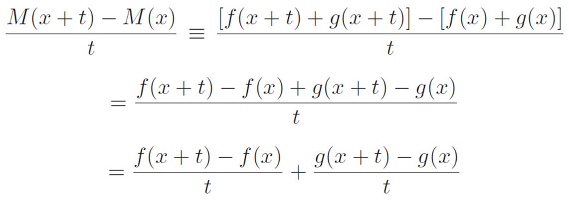
In the first equality we used the definition of M. In the second and third equalities, we were just shuffling things around, trying to segregate the f stuff from the g stuff. We did that because the whole point of all this is to break a hard problem into a bunch of easy problems, so it would be helpful to be able to talk about the derivative of a big machine M just by talking about the derivatives of its parts f and g. It turns out that we’ve managed to do exactly that. If we now imagine shrinking t down closer and closer to zero, the top left of the above equation will turn into M′(x). Similarly, the bottom is made up of two pieces, and when we shrink t down to zero, one of them will morph into f′(x), and the other will morph into g′(x).

So! We just discovered a new fact about our infinite magnifying glass, one that will be helpful in breaking large problems into simpler parts. Let’s give this its own box like we did before, and write the same idea in several different ways.

What We Just Invented

Is there a relationship between the derivatives of a big machine M(x) ≡ f(x) + g(x) and the derivatives of the parts f(x) and g(x) out of which it is built? Yes!

If M(x) = f(x) + g(x), then M′(x) = f′(x) + g′(x)

Let’s say the same thing in a different way:

[f(x) + g(x)]′ = f′(x) + g′(x)

Let’s say the same thing in a different way. . . again!

This is getting crazy, but let’s do it again!

(f + g)′ = f′ + g′

You still there? Okay, one more time!

This might work for any number of machines, but we don’t know yet:

So we discovered how to deal with two machines added together. But what if we have 3 or 100 or n machines added together? Do we need to figure out a new law for each possible number from 2 up? If we think about it for a moment, we can see that this problem goes away as soon as we recognize the power of an idea we mentioned earlier. That idea was this:

The question “How many machines are there really in a big machine?” is a meaningless question. If it helps us to think of a big machine as two smaller machines taped together, then we’re free to think of it that way.

The same philosophy clearly applies to any number of pieces, not necessarily two. If we acknowledge that a bunch of machines taped together also counts as a single “big machine,” then we can pull an interesting trick. Imagine that we have a big machine that we’re thinking of as three pieces added together. What’s the derivative of the big machine? We only know that “the derivative of a sum is the sum of the derivatives” for the simple case of two parts, that is to say:

(f + g)′ = f′ + g′

But if we think of the sum of a bunch of machines as a machine in its own right, then we can just apply the simple two-parts version twice, like this:

[f + g + h]′ = [f + (g + h)]′ = f′ + (g + h)′ = f′ + g′ + h′

The first equality just says “we’re thinking of (f + g) as a single machine, just for a moment.” In the second and third equalities, we used the simpler version that we know already: you can distribute the apostrophes when there are only two parts. First we used it on f and (g + h), thinking of (g + h) as a single machine. Then we used it on g and h, no longer thinking of them as a single machine. So the way we were thinking about (g + h) completely changed in the middle of the equations above. It’s not hard to convince ourselves that this same kind of reasoning can take us as high as we want. Try to convince yourself that if we have n machines, then the following is true:

and that this comes from exactly the same type of reasoning we used to get from two machines to three. We just have to imagine applying the same argument over and over. The consequences of this are fairly amazing, because just by figuring out the “two-parts” version (f + g)′ = f′ + g′, we automatically got a more general version. By using the “two-parts” version and then repeatedly changing our minds about whether we think of something as two machines or as one big machine with two parts, we were able to trick the mathematics into thinking that we had figured out the bigger “n-parts” version!

(A faint rumbling noise is heard in the distance.)

Aaah! It happened again!

Reader: Why do you keep doing that?

Author: It’s not me!

Reader: (Skeptically) . . . Are you sure?

Author: Yes! I don’t know what’s going on any more than you do. . . Where were we? Oh, I think we’re done with this section! Onward, dear Reader!

2.3.8The Last Problem in Our Universe. . . for Now

In the last section we invented the following facts:

and

where # is any number, and M, f, and g are any machines, not necessarily plus-times machines (though we know of no other kind at this point). Also, we found earlier that the derivative of xⁿ is

and we saw that the “two-parts” version (f + g)′ = f′ + g′ was just as powerful as the “n-parts” version:

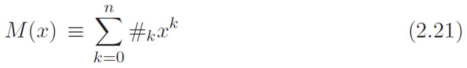
We’ve got all the ingredients in place to figure out how to use our infinite magnifying glass on any plus-times machine (or if you prefer, on all possible plus-times machines at once). Let’s do that! We convinced ourselves earlier that the abbreviation

was large enough and agnostic enough to let us talk about any plus-times machine. Now we know how to talk about the derivative of the whole thing in terms of the derivatives of the pieces, and we know how to figure out the derivatives of each of the pieces. So all we have to do is combine these two discoveries, and we will have mastered our invention as much as it can be mastered. . . at least at this point. That is, at the beginning of the chapter, we invented the infinite magnifying glass, and now if we can manage to solve this last problem of ours, we will have figured out how to apply that invention to all the machines that currently exist in our universe.

In the following argument, we’ll see how helpful it can be to have different kinds of equals signs in a long mathematical sentence. As usual, I’ll use ≡ whenever something is true just because we’re reabbreviating, so you don’t need to worry about why those parts are true. The argument below may look fairly complicated, but a surprising number of steps are just reabbreviation. Three steps won’t be, though. I’ll write 2.19 above the equals sign where we’re using equation 2.19, and I’ll do the same thing for equations 2.16 and 2.18. These are the only things we’ll need. Take a deep breath, and try to follow along. Here we go. . .

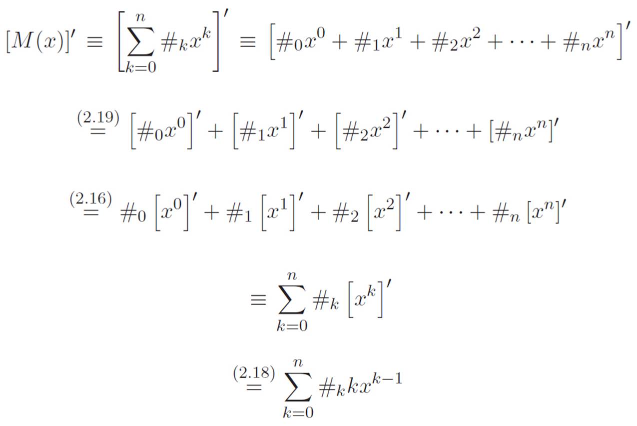
Done! In retrospect, most of those steps weren’t entirely necessary, but I wanted to go as slowly as possible to avoid getting lost in all the symbols. Now that we get the idea, though, we could have made the exact same argument without so many reabbreviations. Here’s what that argument would look like if we made it more casually. We want to differentiate a machine that looks like this:

This is just a sum of a bunch of things. We know from equation 2.19 that the derivative of a sum is just the sum of the individual derivatives, and because of equations 2.16 and 2.18 we know that the derivative of #_kx^k is just #k^kxk−1. So, knowing both of those things, we can make the above argument all in one step, and conclude that the derivative of M is

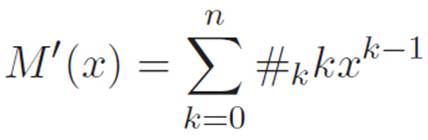
And we’re done again. We’re essentially done with the chapter as well. At least the meat of it. So, since the chapter began, we’ve come up with the idea of an infinite magnifying glass, used it to define a new concept (the derivative), and figured out how to apply that concept to every machine that currently exists in our universe.

Before we officially end the chapter, let’s spend a bit of time in semi-relaxation mode. First, we’ll spend a few pages talking about a new ability we now have as a side effect of our magnifying glass expertise. Then, we’ll briefly discuss the role of “rigor” and “certainty” in mathematics.