Calculus II For Dummies, 2nd Edition (2012)

Part IV. Infinite Series

Chapter 13. Dressing Up Functions with the Taylor Series

In This Chapter

Understanding elementary functions

Seeing power series as polynomials with infinitely many terms

Expressing functions as a Maclaurin series

Discovering the Taylor series as a generalization of the Maclaurin series

The infinite series known as the Taylor series is one of the most brilliant mathematical achievements you’ll ever come across. It’s also quite a lot to get your head around. Although many calculus books tend to throw you in the deep end with the Taylor series, I prefer to take you by the hand and help you wade in slowly.

The Taylor series is a specific form of the power series. In turn, it’s helpful to think of a power series as a polynomial with an infinite number of terms. So, in this chapter, I begin with a discussion of polynomials. I contrast polynomials with other elementary functions, pointing out a few reasons mathematicians like polynomials so much (often to the exclusion of their families and friends).

Then I move on to power series, showing you how to discover when a power series converges and diverges. I also discuss the interval of convergence for a power series, which is the set of x values for which that series converges. After that, I introduce you to the Maclaurin series — a simplified, but powerful, version of the Taylor series.

Finally, the main event: the Taylor series. First, I show you how to use the Taylor series to evaluate other functions; you’ll definitely need that for your final exam. I introduce you to the Taylor remainder term, which allows you to find the margin of error when making an approximation. To finish up the chapter, I show you why the Taylor series works, which helps to make sense of the series, but may not be strictly necessary for passing an exam.

Elementary Functions

Elementary functions are those familiar functions that you work with all the time in calculus. They include:

Addition, subtraction, multiplication, and division

Powers and roots

Exponential functions and logarithms (usually the natural log)

Trig and inverse trig functions

All combinations and compositions of these functions

In this section, I discuss some of the difficulties of working with elementary functions. In contrast, I show you why a small subset of elementary functions — the polynomials — is much easier to work with. To finish, I consider the advantages of expressing elementary functions as polynomials when possible.

Knowing two drawbacks of elementary functions

The set of elementary functions is closed under the operation of differentiation. That is, when you differentiate an elementary function, the result is always another elementary function.

Unfortunately, this set isn’t closed under the operation of integration. For example, here’s an integral that can’t be evaluated as an elementary function:

So even though the set of elementary functions is large and complex enough to confuse most math students, for you — the calculus guru — it’s a rather small pool.

Another problem with elementary functions is that many of them are difficult to evaluate for a given value of x. Even the simple function sin x isn’t so simple to evaluate because (except for 0) every integer input value results in an irrational output for the function. For example, what’s the value of sin 3?

Appreciating why polynomials are so friendly

In contrast to other elementary functions, polynomials are just about the friendliest functions around. Here are just a few reasons:

Polynomials are easy to integrate (see Chapter 4 to see how to compute the integral of every polynomial).

Polynomials are easy to evaluate for any value of x.

Polynomials are infinitely differentiable — that is, you can calculate the value of the first derivative, second derivative, third derivative, and so on, infinitely.

Representing elementary functions as polynomials

In Part II, I show you a set of tricks for computing and integrating elementary functions. Many of these tricks work by taking a function whose integral can’t be computed as such and tweaking it into a more friendly form.

For example, using the substitution u = sin x, you can turn the integral on the left into the one on the right:

In this case, you can turn the product of two trig functions into a polynomial, which is much simpler to work with and easy to integrate.

Representing elementary functions as series

The tactic of expressing complicated functions as polynomials (and other simple functions) motivates much of the study of infinite series.

Although series may seem difficult to work with — and, admittedly, they do pose their own specific set of challenges — they have two great advantages that make them useful for integration:

An infinite series breaks easily into terms. So in most cases, you can use the Sum Rule to break a series into separate terms and evaluate these terms individually.

Series tend to be built from a recognizable pattern. So if you can figure out how to integrate one term, you can usually generalize this method to integrate every term in the series.

Specifically, power series include many of the features that make polynomials easy to work with. I discuss power series in the next section.

Power Series: Polynomials on Steroids

In Chapter 11, I introduce the geometric series:

I also show you a simple formula to figure out whether the geometric series converges or diverges.

The geometric series is a simplified form of a larger set of series called the power series.

A power series is any series of the following form:

Notice how the power series differs from the geometric series:

In a geometric series, every term has the same coefficient.

In a power series, the coefficients may be different — usually according to a rule that’s specified in the sigma notation.

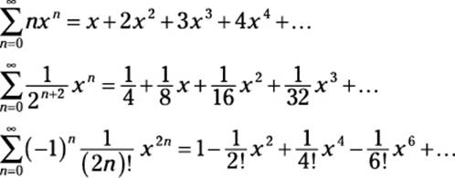
Here are a few examples of power series:

You can think of a power series as a polynomial with an infinite number of terms. For this reason, many useful features of polynomials (which I describe earlier in this chapter) carry over to power series.

The most general form of the power series is as follows:

This form is for a power series that’s centered at a. Notice that when a = 0, this form collapses to the simpler version I introduce earlier in this section. So a power series in this form is centered at 0.

Integrating power series

In Chapter 4, I show you a three-step process for integrating polynomials. Because power series resemble polynomials, they’re simple to integrate using the same basic process:

1. Use the Sum Rule to integrate the series term by term.

2. Use the Constant Multiple Rule to move each coefficient outside its respective integral.

3. Use the Power Rule to evaluate each integral.

For example, take a look at the following integral:

At first glance, this integral of a series may look scary. But to give it a chance to show its softer side, I expand the series out as follows:

Now you can apply the three steps for integrating polynomials to evaluate this integral:

1. Use the Sum Rule to integrate the series term by term:

2. Use the Constant Multiple Rule to move each coefficient outside its respective integral:

3. Use the Power Rule to evaluate each integral:

Notice that this result is another power series, which you can turn back into sigma notation:

Understanding the interval of convergence

As with geometric series and p-series (which I discuss in Chapter 11), an advantage to power series is that they converge or diverge according to a well-understood pattern.

Unlike these simpler series, however, a power series often converges or diverges based on its x value. This leads to a new concept when dealing with power series: the interval of convergence.

The interval of convergence for a power series is the set of x values for which that series converges.

The interval of convergence is never empty

Every power series converges for some value of x. That is, the interval of convergence for a power series is never the empty set.

Although this fact has useful implications, it’s actually pretty much a no-brainer. For example, take a look at the following power series:

When x = 0, this series evaluates to 1 + 0 + 0 + 0 + ..., so it obviously converges to 1. Similarly, take a peek at this power series:

This time, when x = –5, the series converges to 0, just as trivially as the last example.

Note that in both of these examples, the series converges trivially at x = a for a power series centered at a (see the beginning of “Power Series: Polynomials on Steroids”).

Three varieties for the interval of convergence

Three possibilities exist for the interval of convergence of any power series:

The series converges only when x = a.

The series converges on some interval (open or closed at either end) centered at a.

The series converges for all real values of x.

For example, suppose that you want to find the interval of convergence for:

This power series is centered at 0, so it converges when x = 0. Using the ratio test (see Chapter 12), you can find out whether it converges for any other values of x. To start out, set up the following limit:

To evaluate this limit, start out by canceling xⁿ in the numerator and denominator:

Next, distribute to remove the parentheses in the numerator:

As it stands, this limit is of the form , so apply L’Hopital’s Rule (see Chapter 2), differentiating over the variable n:

From this result, the ratio test tells you that the series:

Converges when –1 < x < 1

Diverges when x < –1 and x > 1

May converge or diverge when x = 1 and x = –1

Fortunately, it’s easy to see what happens in these two remaining cases. Here’s what the series looks like when x = 1:

Clearly, the series diverges. Similarly, here’s what it looks like when x = –1:

This alternating series swings wildly between negative and positive values, so it also diverges.

As a final example, suppose that you want to find the interval of convergence for the following series:

As in the last example, this series is centered at 0, so it converges when x = 0. The real question is whether it converges for other values of x. Because this is an alternating series, I apply the ratio test to the positive version of it to see whether I can show that it’s absolutely convergent:

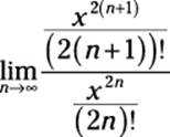
First off, I want to simplify this a bit:

Next, I expand out the exponents and factorials, as I show you in Chapter 12:

At this point, a lot of canceling is possible:

This time, the limit falls between –1 and 1 for all values of x. This result tells you that the series converges absolutely for all values of x, so the alternating series also converges for all values of x.

Expressing Functions as Series

In this section, you begin to explore how to express functions as infinite series. I begin by showing some examples of formulas that express sin x and cos x as series. These examples lead to a more general formula for expressing a wider variety of elementary functions as series.

This formula is the Maclaurin series, a simplified but powerful version of the more general Taylor series, which I introduce later in this chapter.

Expressing sin x as a series

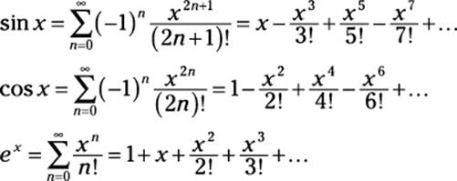
Here’s an odd formula that expresses the sine function as an alternating series:

To make sense of this formula, use expanded notation:

Notice that this is a power series (which I discuss earlier in this chapter). To get a quick sense of how it works, here’s how you can find the value of sin 0 by substituting 0 for x:

As you can see, the formula verifies what you already know: sin 0 = 0.

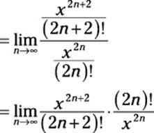
You can use this formula to approximate sin x for any value of x to as many decimal places as you like. For example, look what happens when you substitute 1 for x in the first four terms of the formula:

Note that the actual value of sin 1 to six decimal places is 0.841471, so this estimate is correct to five decimal places — not bad!

Expressing cos x as a series

In the previous section, I show you a formula that expresses the value of sin x for all values of x as an infinite series. Differentiating both sides of this formula leads to a similar formula for cos x:

Now evaluate these derivatives:

Finally, simplify the result a bit:

As you can see, the result is another power series (which I discuss earlier in this chapter). Here’s how you write it with sigma notation:

To gain some confidence that this series really works as advertised, note that the substitution x = 0 provides the correct equation cos 0 = 1. Furthermore, substituting x = 1 into the first four terms gives you the following approximation:

This estimate is accurate to four decimal places.

Introducing the Maclaurin Series

In the previous two sections, I show you formulas for expressing both sin x and cos x as infinite series. You may begin to suspect that there’s some sort of method behind these formulas. Without further ado, here it is:

Behold the Maclaurin series, a simplified version of the much-heralded Taylor series, which I introduce in the next section.

The notation f⁽ⁿ⁾ means “the nth derivative of f.” This should become clearer in the expanded version of the Maclaurin series:

The Maclaurin series is the template for the two formulas I introduce earlier in this chapter. It allows you to express many other functions as power series by following these steps:

1. Find the first few derivatives of the function until you recognize a pattern.

2. Substitute 0 for x into each of these derivatives.

3. Plug these values, term by term, into the formula for the Maclaurin series.

4. If possible, express the series in sigma notation.

For example, suppose that you want to find the Maclaurin series for e^x.

1. Find the first few derivatives of e^x until you recognize a pattern:

f'(x) = e^x

f"(x) = e^x

f(x) = e^x

...

f⁽ⁿ⁾(x) = e^x

2. Substitute 0 for x into each of these derivatives.

f'(0) = e⁰

f"(0) = e⁰

f(0) = e⁰

...

f⁽ⁿ⁾(x) = e⁰

3. Plug these values, term by term, into the formula for the Maclaurin series:

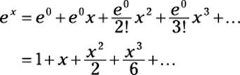
4. If possible, express the series in sigma notation:

To check this formula, use it to estimate e⁰ and e¹ by substituting 0 and 1, respectively, into the first six terms:

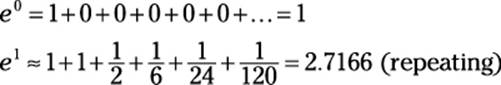
This exercise nails e⁰ exactly, and approximates e¹ to two decimal places. And, as with the formulas for sin x and cos x that I show you earlier in this chapter, the Maclaurin series for e^x allows you to calculate this function for any value of x to any number of decimal places.

As with the other formulas, however, the Maclaurin series for e^x works best when x is close to 0. As x moves away from 0, you need to calculate more terms to get the same level of precision.

But now, you can begin to see why the Maclaurin series tends to provide better approximations for values close to 0: The number 0 is “hardwired” into the formula as f(0), f'(0), f"(0), and so forth.

Figure 13-1 illustrates this point. The first graph shows sin x approximated by using the first two terms of the Maclaurin series — that is, as the third-degree polynomial . The subsequent graph shows an approximation of sin x with four terms.

As you can see, each successive approximation improves on the previous one. Furthermore, each equation tends to provide its best approximation when x is close to 0.

A tale of three series

It’s easy to get confused about the three categories of series that I discuss in this chapter. Here’s a helpful way to think about them:

The power series is a subcategory of infinite series.

The Taylor series (named for mathematician Brook Taylor) is a subcategory of power series.

The Maclaurin series (named for mathematician Colin Maclaurin) is a subcategory of Taylor series.

After you have that down, consider that the power series has two basic forms:

The specific form, which is centered at zero, so a drops out of the expression.

The general form, which isn’t centered at zero, so a is part of the expression.

Furthermore, each of the other two series uses one of these two forms of the power series:

The Maclaurin series uses the specific form, so it’s less powerful and simpler to work with.

The Taylor series uses the general form, so it’s more powerful and harder to work with.

Introducing the Taylor Series

Like the Maclaurin series (which I introduce in the previous section), the Taylor series provides a template for representing a wide variety of functions as power series.

In fact, the Taylor series is really a more general version of the Maclaurin series. The advantage of the Maclaurin series is that it’s a bit simpler to work with. The advantage to the Taylor series is that you can tailor it to obtain a better approximation of many functions.

Here’s the Taylor series in all its glory:

As with the Maclaurin series, the Taylor series uses the notation f⁽ⁿ⁾ to indicate the nth derivative. Here’s the expanded version of the Taylor series:

Notice that the Taylor series includes the variable a, which isn’t found in the Maclaurin series. Or, more precisely, in the Maclaurin series, a = 0, so it drops out of the expression.

The explanation for this variable can be found earlier in this chapter, in “Power Series: Polynomials on Steroids.” In that section, I show you two forms of the power series:

A simpler form centered at 0, which corresponds to the Maclaurin series

A more general form centered at a, which corresponds to the Taylor series

In the next section, I show you the advantages of working with this extra variable.

Computing with the Taylor series

The presence of the variable a makes the Taylor series more complex to work with than the Maclaurin series. But this variable provides the Taylor series with greater flexibility, as the next example illustrates.

In “Expressing Functions as Series” earlier in this chapter, I attempt to approximate the value of sin 10 with the Maclaurin series. Unfortunately, taking this calculation out to eight terms still results in a poor estimate. This problem occurs because the Maclaurin series always takes a default value of a = 0, and 0 isn’t close enough to 10.

This time, I use only four terms of the Taylor series to make a much better approximation. The key to this approximation is a shrewd choice for the variable a:

Let a = 3π

This choice has two advantages: First, this value of a is close to 10 (the value of x), which makes for a better approximation. Second, it’s an easy value for calculating sines and cosines, so the computation shouldn’t be too difficult.

To start off, substitute 10 for x and 3π for a in the first four terms of the Taylor series:

Next, substitute in the first, second, and third derivatives of the sine function and simplify:

The good news is that sin 3π = 0, so the first and third terms fall out:

At this point, you probably want to grab your calculator:

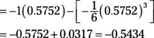
This approximation is correct to two decimal places — quite an improvement over the estimate from the Maclaurin series!

Examining convergent and divergent Taylor series

Earlier in this chapter, I show you how to find the interval of convergence for a power series — that is, the set of x values for which that series converges.

Because the Taylor series is a form of power series, you shouldn’t be surprised that every Taylor series also has an interval of convergence. When this interval is the entire set of real numbers, you can use the series to find the value of f(x) for every real value of x.

However, when the interval of convergence for a Taylor series is bounded — that is, when it diverges for some values of x — you can use it to find the value of f(x) only on its interval of convergence.

For example, here are the three important Taylor series I’ve introduced so far in this chapter:

All three of these series converge for all real values of x (you can check this by using the ratio test, as I show you earlier in this chapter), so each equals the value of its respective function.

Now consider the following function:

I express this function as a Maclaurin series, using the steps that I outline earlier in this chapter in “Expressing Functions as Series”:

1. Find the first few derivatives of until you recognize a pattern:

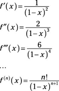
2. Substitute 0 for x into each of these derivatives:

f'(0) = 1

f"(0) = 2

f(0) = 6

...

f⁽ⁿ⁾(0) = n!

3. Plug these values, term by term, into the formula for the Maclaurin series:

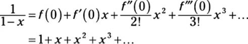
4. If possible, express the series in sigma notation:

To test this formula, I use it to find f(x) when x = .

You can test the accuracy of this expression by substituting into :

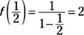
As you can see, the formula produces the correct answer. Now I try to use it

to find f(x) when x = 5, noting that the correct answer should be :

f(5) = 1 + 5 + 25 + 125 + ... = ∞ WRONG!

What happened? This series converges only on the interval (–1, 1), so the formula produces only the value f(x) when x is in this interval. When x is outside this interval, the series diverges, so the formula is invalid.

Expressing functions versus approximating functions

It’s important to be crystal clear in your understanding about the difference between two key mathematical practices:

Expressing a function as an infinite series

Approximating a function by using a finite number of terms of series

Both the Taylor series and the Maclaurin series are variations of the power series. You can think of a power series as a polynomial with infinitely many terms. Also, recall that the Maclaurin series is a specific form of the more general Taylor series, arising when the value of a is set to 0.

Every Taylor series (and, therefore, every Maclaurin series) provides the exact value of a function for all values of x where that series converges. That is, for any value of x on its interval of convergence, a Taylor series converges to f(x).

In practice, however, adding up an infinite number of terms simply isn’t possible. Nevertheless, you can approximate the value of f(x) by adding a finite number from the appropriate Taylor series. You do this earlier in the chapter to estimate the value of sin 10 and other expressions.

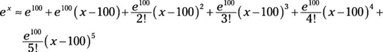
An expression built from a finite number of terms of a Taylor series is called a Taylor polynomial, T_n(x). Like other polynomials, a Taylor polynomial is identified by its degree. For example, here’s the fifth-degree Taylor polynomial, T₅(x), that approximates e^x:

Generally speaking, a higher-degree polynomial results in a better approximation. And because this polynomial comes from the Maclaurin series, where a = 0, it provides a much better estimate for values of e^x when x is near 0. For the value of e^x when x is near 100, however, you get a better estimate by using a Taylor polynomial for e^x with a = 100:

To sum up, remember the following:

A convergent Taylor series expresses the exact value of a function.

A Taylor polynomial, T_n(x), from a convergent series approximates the value of a function.

Calculating error bounds for Taylor polynomials

In the previous section, I discuss how a Taylor polynomial approximates the value of a function:

In many cases, it’s helpful to measure the accuracy of an approximation. This information is provided by the Taylor remainder term:

f(x) = T_n(x) + R_n(x)

Notice that the addition of the remainder term R_n(x) turns the approximation into an equation. Here’s the formula for the remainder term:

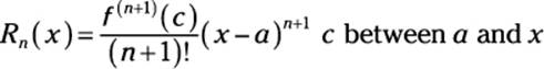
It’s important to be clear that this equation is true for one specific value of c on the interval between a and x. It does not work for just any value of c on that interval.

Ideally, the remainder term gives you the precise difference between the value of a function and the approximation T_n(x). However, because the value of c is uncertain, in practice the remainder term really provides a worst-case scenario for your approximation.

An example should help to make this idea clear. I use the sixth-degree Taylor polynomial for cos x:

Suppose that I use this polynomial to approximate cos 1:

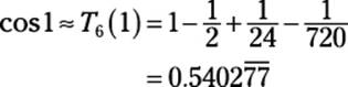
How accurate is this approximation likely to be? To find out, use the remainder term:

cos 1 = T₆(x) + R₆(x)

Adding the associated remainder term changes this approximation into an equation. Here’s the formula for the remainder term:

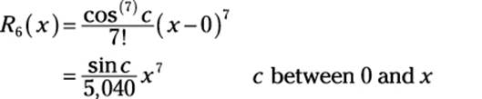
So substituting 1 for x gives you:

At this point, you’re apparently stuck, because you don’t know the value of sin c. However, you can plug in c = 0 and c = 1 to give you a range of possible values:

This simplifies to provide a very close approximation:

0 ≤ R₆ (1) ≤ 0.00017

Thus, the remainder term predicts that the approximate value calculated above will be within 0.00017 of the actual value. And, in fact, , so:

As you can see, the approximation is within the error bounds predicted by the remainder term.

Understanding Why the Taylor Series Works

The best way to see why the Taylor series works is to see how it’s constructed in the first place. If you read through this chapter until this point, you should be ready to go.

To make sure that you understand every step along the way, however, I construct the Maclaurin series, which is just a tad more straightforward. This construction begins with the key assumption that a function can be expressed as a power series in the first place:

f(x) = c₀ + c₁x + c₂x² + c₃x³ + ...

The goal now is to express the coefficients on the right side of this equation in terms of the function itself. To do this, I make another relatively safe assumption that 0 is in the domain of f(x). So when x = 0, all but the first term of the series equal 0, leaving the following equation:

f(0) = c₀

This process gives you the value of the coefficient c₀ in terms of the function. Now differentiate f(x):

f'(x) = c₁ + 2c₂x + 3c₃x² + 4c₄x³...

At this point, when x = 0, all the x terms drop out:

f'(0) = c₁

So you have another coefficient, c₁, expressed in terms of the function. To continue, differentiate f'(x):

f"(x) = 2c₂ + 6c₃x + 12c₄x² + 20c₅x³ + ...

Again, when x = 0, the x terms disappear:

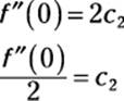
By now, you’re probably noticing a pattern: You can always get the value of the next coefficient by differentiating the previous equation and substituting 0 for x into the result:

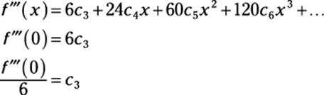
Furthermore, the coefficients also have a pattern:

Substituting these coefficients into the original equation results in the familiar Maclaurin series from earlier in this chapter:

To construct the Taylor series, use a similar line of reasoning, starting with the more general form of the power series:

f(x) = c₀ + c₁(x – a) + c₂(x – a)² + c₃(x – a)³ + ...

In this case, setting x = a gives you the first coefficient:

f(a) = c₀

Continue to find coefficients by differentiating f(x) and then repeating the process.