Calculus II For Dummies, 2nd Edition (2012)

Part V. Advanced Topics

Chapter 15. What’s So Different about Differential Equations?

In This Chapter

Classifying different types of differential equations (DEs)

Understanding the connection between DEs and integrals

Checking a proposed solution to a DE

Seeing how DEs arise in the physical world

The very mention of differential equations (DEs for short) strikes a spicy combination of awe, horror, and utter confusion into nonmathematical minds. Even intrepid calculus students have been known to consider a career in art history when these untamed beasts come into focus on the radar screen. Just what are differential equations? Where do they come from? Why are they necessary? And how in the world do you solve them?

In this chapter, I answer these questions and give you some familiarity with DEs. I show you how to identify the basic types of DEs so that if you’re ever at a math department cocktail party (lucky you!), you won’t feel completely adrift. I relate DEs to the integrals that you discover earlier in the book. I show you how to build your own DEs so you’ll always have a hobby to pass the time, and I also show you how to check DE solutions. In addition, you discover how DEs arise in physics. Finally, I show you a few simple methods for solving some basic differential equations.

Basics of Differential Equations

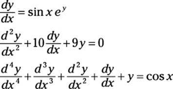
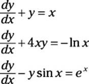
In a nutshell, a differential equation, or DE, is any equation that includes at least one derivative. For example:

Solving a differential equation means finding the value of the dependent variable in terms of the independent variable. Throughout this chapter, I use y as the dependent variable, so the goal in each problem is to solve for y in terms of x.

In this section, I show you how to classify DEs. I also show you how to build DEs and check the solution to a DE.

Classifying DEs

As with other equations that you’ve encountered, differential equations come in many varieties. And different varieties of DEs can be solved using different methods. In this section, I show you some important ways to classify DEs.

Ordinary and partial differential equations

An ordinary differential equation (ODE) has only derivatives of one variable — that is, it has no partial derivatives (flip to Chapter 14 for more on partial differentiation). Here are a few examples of ODEs:

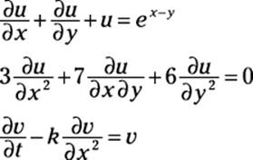
In contrast, a partial differential equation (PDE) has at least one partial derivative. Here are a few examples of PDEs:

Ordinary differential equations are usually the topic of a typical Differential Equations class in college. They’re a step or two beyond what you’re used to working with, but many students actually find Differential Equations an easier course than Calculus II (generally considered the most difficult class in the calculus series). However, ODEs are limited in how well they can actually express physical reality.

The real quarry is partial differential equations. A lot of physics gets done with these little gems. Unfortunately, solving PDEs is one giant leap forward in math from what the average calculus student is used to. Delving into the kind of math that makes PDEs come alive is typically reserved for graduate school.

Order of DEs

Differential equations are further classified according to their order. This classification is similar to the classification of polynomial equations by degree (see Chapter 2 for more on polynomials).

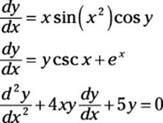
First-order ODEs contain only first derivatives. For example:

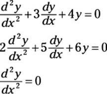
Higher-order ODEs are classified, as polynomials are, by the greatest order of their derivatives. Here are examples of second-, third-, and fourth-order ODEs:

Second-order ODE:

Third-order ODE:

Fourth-order ODE:

As with polynomials, generally speaking, a higher-order DE is more difficult to solve than one of lower order.

Linear DEs

What constitutes a linear differential equation depends slightly on who you ask. For practical purposes, a linear first-order DE fits into the following form:

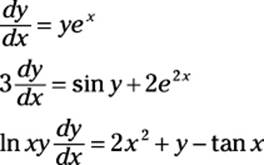
where a(x) and b(x) are functions of x. Here are a few examples of linear first-order DEs:

Linear DEs can often be solved, or at least simplified, using an integrating factor. I show you how to do this later in the chapter.

A linear second-degree DE fits into the following form:

where a, b, and c are all constants. Here are some examples:

Note that the constant a can always be reduced to 1, resulting in adjustments to the other two coefficients. Linear second-degree DEs are usually an important topic in a college-level course in differential equations. Solving them requires knowledge of matrices and complex numbers that is beyond the scope of this book.

Looking more closely at DEs

You don’t have to play professional baseball to enjoy baseball. Instead, you can enjoy the game from the bleachers or, if you prefer, from a nice cushy chair in front of the TV. Similarly, you don’t have to get too deep into differential equations to gain a general understanding of how they work. In this section, I give you front-row seats to the game of differential equations.

How every integral is a DE

The integral is a particular example of a more general type of equation — the differential equation. To see how this is so, suppose that you’re working with this nice little integral:

Differentiating both sides turns it into a DE:

Of course, you know how to solve this DE by thinking of it as an integral:

y = sin x + C

So in general, when a DE is of the form

with f(x) an arbitrary function of x, you can express that DE as an integral and solve it by integrating.

Why building DEs is easier than solving them

The reason that the DE in the last section is so simple to solve is that the derivative is isolated on one side of the equation. DEs attain a new level of difficulty when the derivative isn’t isolated.

A good analogy can be made in lower math, when you make the jump from arithmetic to algebra. For example, here’s an arithmetic problem:

x = 20 – (4² + 3)

Even though this is technically an algebra problem, you can solve it without algebra because x is isolated at the start of the problem. However, the ballgame changes when x becomes more enmeshed in the equation. For example:

2x³ – x² + 5x – 17 = 0

Arithmetic isn’t strong enough for this problem, so algebra takes over. Similarly, when derivatives get entangled into the fabric of an equation — as in most of the DEs I show you earlier in “Classifying DEs” — integrating is no longer effective and the search for new methods begins.

Although solving DEs is often tricky, building them is easy. For example, suppose you start with this simple quadratic equation:

y = 3x² + 4x – 5

Now find the first and second derivatives:

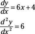
Adding up the left and right sides of all three equations gives you the following differential equation:

Because you built the equation yourself, you know what y equals. But if you hand this equation off to some other students, they probably wouldn’t be able to guess how you built it, so they would have to do some work to solve it for y. For example, here’s another DE:

This equation probably looks difficult because you don’t have much information. And yet, after I tell you the solution, it appears simple:

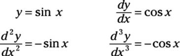
But even after you have the solution, how do you know whether it’s the only solution? For starters, y = –sin x, y = cos x, and y = –cos x are all solutions. Do other solutions exist? How do you find them? And how do you know when you have them all?

Another difficulty arises when y itself becomes tangled up in the equation. For example, how do you solve this equation for y?

As you can see, differential equations contain treacherous subtleties that you don’t find in basic calculus.

Checking DE solutions

Even if you don’t know how to find a solution to a differential equation, you can always check whether a proposed solution works. This is simply a matter of plugging the proposed value of the dependent variable — I use ythroughout this chapter — into both sides of the equation to see whether equality is maintained.

For example, here’s a DE:

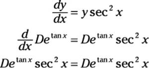
You may not have a clue how to begin solving this DE, but imagine that an angel lands on your pen and offers you this solution:

y = 4e^3x sin x

You can check to see whether this angel really knows math by plugging in this value of y as follows:

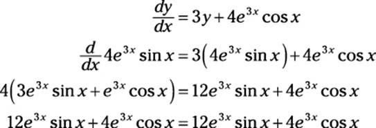
Because the left and right sides of the equation are equal, the angel’s solution checks out.

Solving Differential Equations

In this section, I show you how to solve a few types of DEs. First, you solve everybody’s favorite DE, the separable equation. Next, you put this understanding to work to solve an initial-value problem (IVP). Finally, I show you how to solve a linear first-order DE using an integrating factor.

Solving separable equations

Differential equations become harder to solve the more entangled they become. In certain cases, however, an equation that looks all tangled up is actually easy to tease apart. Equations of this kind are called separable equations(or autonomous equations), and they fit into the following form:

Separable equations are relatively easy to solve. For example, suppose that you want to solve the following problem:

You can think of the symbol as a fraction and isolate the x and y terms of

this equation on opposite sides of the equal sign:

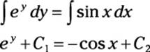
e^y dy = sin x dx

Now integrate both sides:

In an important sense, the previous step is questionable because the variable of integration is different on each side of the equal sign. You may think “No problem, it’s all integration!” But imagine if you tried to divide one side of an equation by 2 and the other by 3, and then laughed it off with “It’s all division!” Clearly, you’d have a problem. The good news, however, is that, for technical reasons beyond the scope of this book, integrating both sides by different variables actually produces the correct answer.

C₁ and C₂ are both constants, so you can use the equation C = C₂ – C₁ to simplify the equation:

e^y = –cos x + C

Next, use a natural log to undo the exponent, and then simplify:

ln e ^y = ln (–cos x + C)

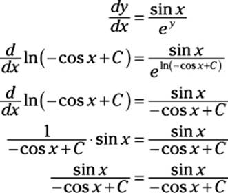
y = ln (–cos x + C)

To check this solution, substitute this value for y into both sides of the original equation:

Solving initial-value problems (IVPs)

In Chapter 3, I show you that the definite integral is a particular example of a whole family of indefinite integrals. In a similar way, an initial-value problem (IVP) is a particular example of a solution to a differential equation. Every IVP gives you extra information — called an initial value — that allows you to use the general solution to a DE to obtain a particular solution.

For example, here’s an initial-value problem:

This problem includes not only a DE but also an additional equation. To understand what this equation tells you, remember that y is a dependent variable, a function of x. So the notation y(0) = 5 means “when x = 0, y = 5.” You see how this information comes into play as I continue with this example.

To solve an IVP, you first have to solve the DE. Do this by finding its general solution without worrying about the initial value. Fortunately, this DE is a separable equation, which you know how to solve from the last section:

Integrate both sides:

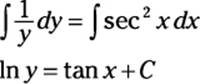
In this last step, I use C to consolidate the constants of integration from both sides of the equation into a single constant C. (If this doesn’t make sense, I explain why in “Solving separable equations” earlier in this chapter.) Next, I undo the natural log by using e:

e^{ln y} = e^{tan x + C}

y = e^{tan x} · e^C

Because e^C is a constant, this equation can be further simplified using the substitution D = e^C:

y = De^{tan x}

Before moving on, check to make sure that this solution is correct by substituting this value of y into both sides of the original equation:

This checks out, so y = De^{tan x} is, indeed, the general solution to the DE. To solve the initial-value problem, however, I need to find the specific value of the variable D by using the additional information I have: When x = 0, y = 5. Plugging both of these values into the equation makes it possible to solve for D:

5 = De^{tan 0}

5 = De⁰

5 = D

Now plug this value of D back into the general solution of the problem to get the IVP solution:

y = 5e^{tan x}

This solution satisfies not only the differential equation but also the initial value y(0) = 5.

Using an integrating factor

As I mention earlier in this chapter, in “Classifying DEs,” a linear first-order equation takes the following form:

A clever method for solving DEs in this form involves multiplying the entire equation by an integrating factor. Follow these steps:

1. Calculate the integrating factor.

2. Multiply the DE by this integrating factor.

3. Restate the left side of the equation as a single derivative.

4. Integrate both sides of the equation and solve for y.

Don’t worry if these steps don’t mean much to you. In the upcoming sections, I show you what an integrating factor is and how to use it to solve linear first-order DEs.

Getting very lucky

To help you understand how multiplying by an integrating factor works, I set up an equation that practically solves itself — that is, if you know what to do:

Notice that this is a linear first-degree DE, with and b(x) = 0. I now tweak this equation by multiplying every term by x² (you see why shortly):

Next, I use algebra to do a little simplifying and rearranging:

Here’s where I appear to get extremely lucky: The two terms on the left side of the equation just happen to be the result of the application of the Product Rule to the expression y · x² (for more on the Product Rule, see Chapter 2):

Notice that the right side of this equation is exactly the same as the left side of the previous equation. So I can make the following substitution:

Now, to undo the derivative on the left side, I integrate both sides, and then I solve for y:

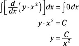
To check this solution, I plug this value of y back into the original equation:

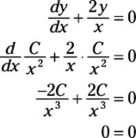
Making your luck

The previous example works because I found a way to multiply the entire equation by a factor that made the left side of the equation look like a derivative resulting from the Product Rule. Although this looked lucky, if you know what to multiply by, every linear first-order DE can be transformed in this way. Recall that the form of a linear first-order DE is as follows:

The trick is to multiply the DE by an integrating factor based on a(x). Here’s the integrating factor:

How the integrating factor is originally derived is beyond the scope of this book. All you need to know here is that it works.

For example, in the previous problem, you know that . So here’s how to find the integrating factor:

Remember that 2 ln x = ln x², so:

As you can see, the integrating factor x² is the exact value that I multiplied by to solve the problem. To see how this process works now that you know the trick, here’s another DE to solve:

In this case, a(x) = 3, so compute the integrating factor as follows:

Now multiply every term in the equation by this factor:

If you like, use algebra to simplify the right side and rearrange the left side:

Now you can see how the left side of this equation looks like the result of the Product Rule applied to evaluate the following derivative:

Because the right side of this equation is the same as the left side of the previous equation, I can make the following substitution:

Notice that I change the left side of the equation using the Product Rule in reverse. That is, I’m expressing the whole left side as a single derivative. Now I can integrate both sides to undo this derivative:

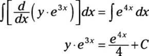
Now solve for y and simplify:

To check this answer, substitute this value of y back into the original DE:

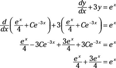
As if by magic, this answer checks out, so the solution is valid.