Calculus II For Dummies, 2nd Edition (2012)

Part II. Indefinite Integrals

Chapter 8. When All Else Fails: Integration with Partial Fractions

In This Chapter

Rewriting complicated fractions as the sum of two or more partial fractions

Knowing how to use partial fractions in four distinct cases

Integrating with partial fractions

Let’s face it: At this point in your math career, you have bigger things to worry about than adding a couple of fractions. And if you’ve survived integration by parts (Chapter 6) and trig integration (Chapter 7), multiplying a few polynomials isn’t going to kill you either.

So here’s the good news about partial fractions: They’re based on simple arithmetic and algebra. In this chapter, I introduce you to the basics of partial fractions and show you how to use them to evaluate integrals. I illustrate four separate cases in which partial fractions can help you integrate functions that would otherwise be a big ol’ mess.

Now here’s the bad news: Although the concept of partial fractions isn’t difficult, using them to integrate is just about the most tedious thing you encounter in this book. And as if that weren’t enough, partial fractions only work with proper rational functions, so I show you how to distinguish these from their ornery cousins, improper rational functions. I also give you a big blast from the past, a refresher on polynomial division, which I promise is easier than you remember it to be.

Strange but True: Understanding Partial Fractions

Partial fractions are useful for integrating rational functions — that is, functions in which a polynomial is divided by a polynomial. The basic tactic behind partial fractions is to split up a rational function that you can’t integrate into two or more simpler functions that you can integrate.

In this section, I show you a simple analogy for partial fractions that involves only arithmetic. After you understand this analogy, partial fractions make a lot more sense. At the end of the section, I show you how to solve an integral using partial fractions.

Looking at partial fractions

Suppose that you want to split the fraction into a sum of two smaller fractions. Start by decomposing the denominator down to its factors — 3 and 5 — and setting the denominators of these two smaller fractions to these numbers:

So you want to find an A and a B that satisfy this equation:

5A + 3B = 14

Now, just by eyeballing this fraction, you can probably find the nice integer solution A = 1 and B = 3, so:

If you include negative fractions, you can find integer solutions like this for

every fraction. For example, the fraction seems too small to be a sum of thirds and fifths, until you discover:

Using partial fractions with rational expressions

The technique of breaking up fractions works for rational expressions. It can provide a strategy for integrating functions that you can’t compute directly. For example, suppose that you’re trying to find this integral:

You can’t integrate this function directly, but if you break it into the sum of two simpler rational expressions, you can use the Sum Rule to solve them separately. And, fortunately, the polynomial in the denominator factors easily:

So set up this polynomial fraction just as I do with the regular fractions in the previous section:

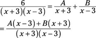
This gives you the following equation:

A(x – 3) + B(x + 3) = 6

This equation works for all values of x. You can exploit this fact to find the values of A and B by picking helpful values of x. To solve this equation for A and B, substitute the roots of the original polynomial (3 and –3) for x and watch what happens:

A(3 – 3) + B(3 + 3) = 6 A(–3 – 3) + B(–3 + 3) = 6

6B = 6 –6A = 6

B = 1 A = –1

Now substitute these values of A and B back into the rational expressions:

This sum of two rational expressions is a whole lot friendlier to integrate than what you started with. Use the Sum Rule followed by a simple variable substitution (see Chapter 5):

= –ln |x + 3| + ln |x – 3| + C

As with regular fractions, you can’t always break rational expressions apart in this fashion. But in four distinct cases, which I discuss in the next section, you can use this technique to integrate complicated rational functions.

Solving Integrals by Using Partial Fractions

In the previous section, I show you how to use partial fractions to split a complicated rational function into several smaller and more-manageable functions. Although this technique will certainly amaze your friends, you may be wondering why it’s worth learning.

The payoff comes when you start integrating. Lots of times, you can integrate a big rational function by breaking it into the sum of several bite-sized chunks. Here’s a bird’s-eye view of how to use partial fractions to integrate a rational expression:

1. Set up the rational expression as a sum of partial fractions with unknowns (A, B, C, and so forth) in the numerators.

I call these unknowns rather than variables to distinguish them from x, which remains a variable for the whole problem.

2. Find the values of all the unknowns and plug them into the partial fractions.

3. Integrate the partial fractions separately by whatever method works.

In this section, I focus on these three steps. I show you how to turn a complicated rational function into a sum of simpler rational functions and how to replace unknowns (such as A, B, C, and so on) with numbers. Finally, I give you a few important techniques for integrating the types of simpler rational functions that you often see when you use partial fractions.

Setting up partial fractions case by case

Setting up a sum of partial fractions isn’t difficult, but you have four distinct cases to watch out for. Each case results in a different setup — some easier than others.

Try to become familiar with these four cases, because I use them throughout this chapter. Your first step in any problem that involves partial fractions is to recognize which case you’re dealing with so that you can solve the problem.

Each of these cases is listed in Table 8-1.

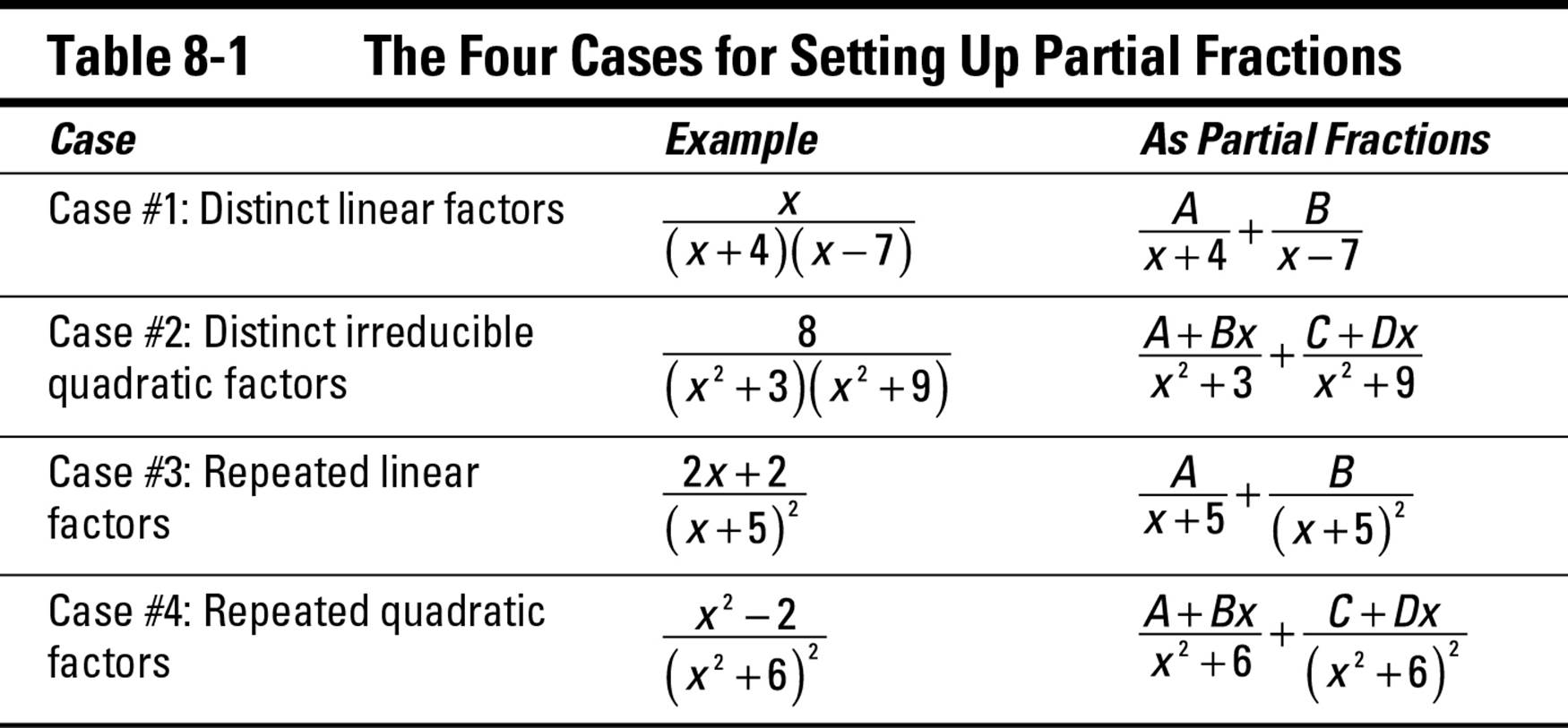
Case #1: Distinct linear factors

The simplest case in which partial fractions are helpful is when the denominator is the product of distinct linear factors — that is, linear factors that are nonrepeating.

For each distinct linear factor in the denominator, add a partial fraction of the following form:

For example, suppose that you want to integrate the following rational expression:

The denominator is the product of three distinct linear factors — x, (x + 2), and (x – 5) — so it’s equal to the sum of three fractions with these factors as denominators:

The number of distinct linear factors in the denominator of the original expression determines the number of partial fractions. In this example, the presence of three factors in the denominator of the original expression yields three partial fractions.

Case #2: Distinct quadratic factors

Another not-so-bad case where you can use partial fractions is when the denominator is the product of distinct quadratic factors — that is, quadratic factors that are nonrepeating.

For each distinct quadratic factor in the denominator, add a partial fraction of the following form:

For example, suppose that you want to integrate this function:

The first factor in the denominator is linear, but the second is quadratic and can’t be decomposed to linear factors. So set up your partial fractions as follows:

As with distinct linear factors, the number of distinct quadratic factors in the denominator tells you how many partial fractions you get. So in this example, two factors in the denominator yield two partial fractions.

Case #3: Repeated linear factors

Repeated linear factors are more difficult to work with because each factor requires more than one partial fraction.

For each squared linear factor in the denominator, add two partial fractions in the following form:

For each quadratic factor in the denominator that’s raised to the third power, add three partial fractions in the following form:

Generally speaking, when a linear factor is raised to the nth power, add n partial fractions. For example, suppose that you want to integrate the following expression:

This expression contains all linear factors, but one of these factors (x + 5) is nonrepeating and the other (x – 1) is raised to the third power. Set up your partial fractions this way:

As you can see, I add one partial fraction to account for the nonrepeating factor and three to account for the repeating factor.

Case #4: Repeated quadratic factors

Your worst nightmare when it comes to partial fractions is when the denominator includes repeated quadratic factors.

For each squared quadratic factor in the denominator, add two partial fractions in the following form:

For each quadratic factor in the denominator that’s raised to the third power, add three partial fractions in the following form:

Generally speaking, when a quadratic factor is raised to the nth power, add n partial fractions. For example:

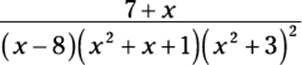
This denominator has one nonrepeating linear factor (x – 8), one nonrepeating quadratic factor (x² + x + 1), and one quadratic expression that’s squared (x² + 3). Here’s how you set up the partial fractions:

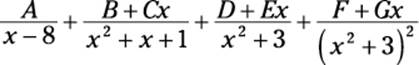
This time, I added one partial fraction for each of the nonrepeating factors and two partial fractions for the squared factor.

Beyond the four cases: Knowing how to set up any partial fraction

At the outset, I have some great news: You’ll probably never have to set up a partial fraction any more complex than the one that I show you in the previous section. So relax.

I’m aware that some students like to get this stuff on a case-by-case basis, so that’s why I introduce it that way. However, other students prefer to be shown an overall pattern so they can get the Zen math experience. If this is your path, read on. If not, feel free to skip ahead.

You can break any rational function into a sum of partial fractions. You just need to understand the pattern for repeated higher-degree polynomial factors in the denominator. This pattern is simplest to understand with an example. Suppose that you’re working with the following rational function:

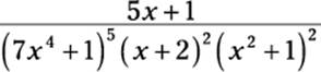
In this factor, the denominator includes a problematic factor that’s a fourth-degree polynomial raised to the fifth power. You can’t decompose this factor further, so the function falls outside the four cases I outline earlier in this chapter. Here’s how you break this rational function into partial fractions:

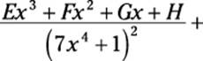
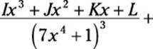
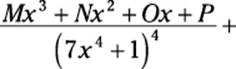
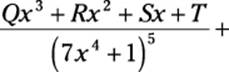
As you can see, I completely run out of capital letters. As you can also see, the problematic factor spawns five partial fractions — that is, the same number as the power it’s raised to. Furthermore:

The numerator of each of these fractions is a polynomial of one degree less than the denominator.

The denominator of each of these fractions is a carbon copy of the original denominator, but in each case raised to a different power up to and including the original.

The remaining two factors in the denominator — a repeated linear (Case #3) and a repeated quadratic (Case #4) — give you the remaining four fractions, which look tiny and simple by comparison.

Clear as mud? Spend a little time with this example and the pattern should become clearer. Notice, too, that the four cases that I outline earlier in this chapter all follow this same general pattern.

You’ll probably never have to work with anything as complicated as this — let alone try to integrate it! — but when you understand the pattern, you can break any rational function into partial fractions without worrying which case it is.

Knowing the ABCs of finding unknowns

You have two ways to find the unknowns in a sum of partial fractions. The easy and quick way is by using the roots of polynomials. Unfortunately, this method doesn’t always find all the unknowns in a problem, though it often finds a few of them. The second way is to set up a system of equations.

Rooting out values with roots

When a sum of partial fractions has linear factors (either distinct or repeated), you can use the roots of these linear factors to find the values of unknowns. For example, in the earlier section “Case #1: Distinct linear factors,” I set up the following equation:

To find the values of the unknowns A, B, and C, first get a common denominator on the right side of this equation (the same denominator that’s on the left side):

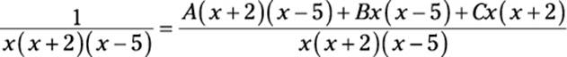
Now multiply both sides by this denominator:

1 = A(x + 2)(x – 5) + Bx(x – 5) + Cx(x + 2)

To find the values of A, B, and C, substitute the roots of the three factors (0, –2, and 5):

1 = A(2)(–5) 1 = B(–2)(–2 – 5) 1 = C(5)(5 + 2)

Plugging these values back into the original equation gives you:

This expression is equivalent to what you started with, but it’s much easier to integrate. To do so, use the Sum Rule to break it into three integrals, the Constant Multiple Rule to move fractional coefficients outside each integral, and variable substitution (see Chapter 5) to do the integration. Here’s the answer so you can try it out:

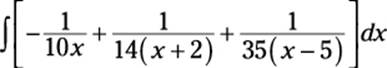
In this answer, I use K rather than C to represent the constant of integration to avoid confusion, because I already use C in the earlier partial fractions.

Working systematically with a system of equations

Setting up a system of equations is an alternative method for finding the value of unknowns when you’re working with partial fractions. It’s not as simple as plugging in the roots of factors (which I show you in the previous section), but it’s your only option when the root of a quadratic factor is imaginary.

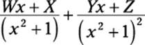
To illustrate this method and why you need it, I use the problem that I set up in “Case #2: Distinct quadratic factors”:

To start out, see how far you can get by plugging in the roots of equations. As I show you in “Rooting out values with roots,” begin by getting a common denominator on the right side of the equation:

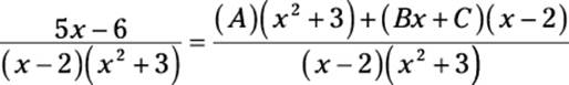
Now multiply the whole equation by the denominator:

5x – 6 = (A)(x² + 3) + (Bx + C)(x – 2)

The root of x – 2 is 2, so let x = 2 and see what you get:

5(2) – 6 = A(2² + 3)

Now you can substitute for A:

Unfortunately, x² + 3 has no root in the real numbers, so you need a different approach. First, get rid of the parentheses on the right side of the equation:

Next, combine similar terms (using x as the variable by which you judge similarity). This is just algebra, so I skip a few steps here:

Because this equation works for all values of x, I now take what appears to be a questionable step, breaking this equation into three separate equations as follows:

–2B + C – 5 = 0

At this point, a little algebra tells you that and . So you can substitute the values of A, B, and C back into the partial fractions:

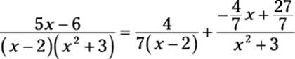
You can simplify the second fraction a bit:

Integrating partial fractions

After you express a hairy rational expression as the sum of partial fractions, integrating becomes a lot easier. Generally speaking, here’s the system:

1. Split all rational terms with numerators of the form Ax + B into two terms.

2. Use the Sum Rule to split the entire integral into many smaller integrals.

3. Use the Constant Multiple Rule to move coefficients outside each integral.

4. Evaluate each integral by whatever method works.

Linear factors: Cases #1 and #3

When you start out with a linear factor — whether distinct (Case #1) or repeated (Case #3) — using partial fractions leaves you with an integral in the following form:

Integrate all these cases by using the variable substitution u = ax + b so that du = a dx and This substitution results in the following integral:

Here are a few examples:

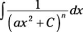
Quadratic factors of the form (ax² + C): Cases #2 and #4

When you start out with a quadratic factor of the form (ax² + C) — whether distinct (Case #2) or repeated (Case #4) — using partial fractions results in the following two integrals:

Integrate the first by using the variable substitution u = ax² + C so that du = 2axdx and du = 2ax dx. This substitution results in the following integral:

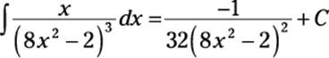
This is the same integral that arises in the linear case that I describe in the previous section. Here are some examples:

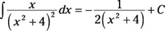
To evaluate the second integral, use the following formula:

Quadratic factors of the form (ax² + bx + C): Cases #2 and #4

Most math teachers have at least a shred of mercy in their hearts, so they don’t tend to give you problems that include this most difficult case. When you start out with a quadratic factor of the form (ax² + bx + C) — whether distinct (Case #2) or repeated (Case #4) — using partial fractions results in the following integral:

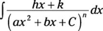
I know, I know — that’s way too many letters and not nearly enough numbers. Here’s an example:

This is about the hairiest integral you’re ever going to see at the far end of a partial fraction. To evaluate it, you want to use the variable substitution u = x² + 6x + 13 so that du = (2x + 6) dx. If the numerator were 2x + 6, you’d be in great shape. So you need to tweak the numerator a bit. First multiply it by 2 and divide the whole integral by 2:

Because you multiplied the entire integral by 1, no net change has occurred. Now add 16 and –16 to the numerator:

This time, you add 0 to the integral, which doesn’t change its value. At this point, you can split the integral in two:

At this point, you can use the desired variable substitution (which I mention a few paragraphs earlier) to change the first integral as follows:

= ln |u| + C

= ln |x² + 6x + 13| + C

To solve the second integral, complete the square in the denominator: Divide the b term (6) by 2 and square it, and then represent the C term (13) as the sum of this and whatever’s left:

Now split the denominator into two squares:

To evaluate this integral, use the same formula that I show you in the previous section:

So here’s the final answer for the second integral:

Therefore, piece together the complete answer as follows:

Integrating Improper Rationals

Integration by partial fractions works with proper rational expressions but not with improper rational expressions. In this section, I show you how to tell these two beasts apart. Then I show you how to use polynomial division to turn improper rationals into more acceptable forms. Finally, I walk you through an example in which you integrate an improper rational expression by using everything in this chapter.

Distinguishing proper and improper rational expressions

Telling a proper fraction from an improper one is easy: A fraction is proper if the numerator (disregarding sign) is less than the denominator, and it’s improper otherwise.

With rational expressions, the idea is similar, but instead of comparing the value of the numerator and denominator, you compare their degrees. The degree of a polynomial is its highest power of x (flip to Chapter 2 for a refresher on polynomials).

A rational expression is proper if the degree of the numerator is less than the degree of the denominator, and it’s improper otherwise.

For example, look at these three rational expressions:

In the first example, the numerator is a second-degree polynomial and the denominator is a third-degree polynomial, so the rational is proper. In the second example, the numerator is a fifth-degree polynomial and the denominator is a second-degree polynomial, so the expression is improper. In the third example, the numerator and denominator are both fourth-degree polynomials, so the rational function is improper.

Recalling polynomial division

Most math students learn polynomial division in Algebra II, demonstrate that they know how to do it on their final exam, and then promptly forget it. And, happily, they never need it again — except to pass the time at extremelydull parties — until Calculus II.

It’s time to take polynomial division out of mothballs. In this section, I show you everything you forgot to remember about polynomial division, both with and without a remainder.

Polynomial division without a remainder

When you multiply two polynomials, you always get another polynomial. For example:

(x³ + 3)(x² – x) = x⁵ – x⁴ + 3x² – 3x

Because division is the inverse of multiplication, the following equation makes intuitive sense:

Polynomial division is a reliable method for dividing one polynomial by another. It’s similar to long division, so you probably won’t have too much difficulty understanding it even if you’ve never seen it.

The best way to show you how to do polynomial division is with an example. Start with the example I’ve already outlined. Suppose that you want to divide x⁵ – x⁴ + 3x² – 3x by x³ + 3. Begin by setting up the problem as a typical long division problem (notice that I fill with zeros for the x³ and constant terms):

Start by focusing on the highest degree exponent in both the divisor (x³) and dividend (x⁵). Ask how many times x³ goes into x⁵ — that is, x⁵ ÷ x³ = ? Place the answer in the quotient, and then multiply the result by the divisor as you would with long division:

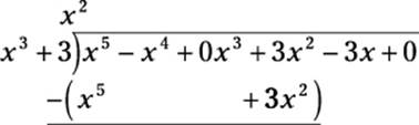
As you can see, I multiply x² by x³ to get the result of x⁵ + 3x², aligning this result to keep terms of the same degree in similar columns. Next, subtract and bring down the next term, just as you would with long division:

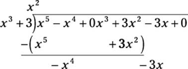
Now the cycle is complete, and you ask how many times x³ goes into –x⁴ — that is, –x⁴ ÷ x³ = ? Place the answer in the quotient, and multiply the result by the divisor:

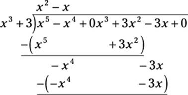
In this case, the subtraction that results works out evenly. Even if you bring down the final zero, you have nothing left to divide, which shows the following equality:

Polynomial division with a remainder

Because polynomial division looks so much like long division, it makes sense that polynomial division should, at times, leave a remainder. For example, suppose that you want to divide x⁴ – 2x³ + 5x by 2x² – 6:

This time, I fill in two zero coefficients as needed. To begin, divide x⁴ by 2x², multiply through, and then subtract:

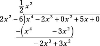
Don’t let the fractional coefficient deter you. Sometimes polynomial division results in fractional coefficients.

Now bring down the next term (5x) to begin another cycle. Then, divide –2x³ by 2x², multiply through, and subtract:

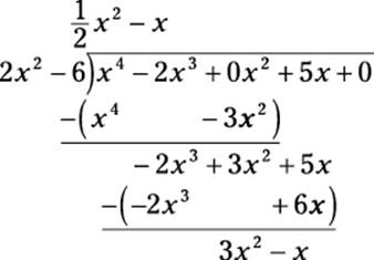
Again, bring down the next term (0) and begin another cycle by dividing 3x² by 2x²:

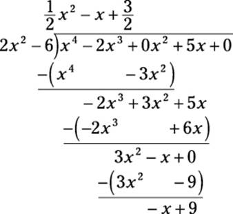
As with long division, the remainder indicates a fractional amount left over: the remainder divided by the divisor. So when you have a remainder in polynomial division, you write the answer using the following formula:

If you get confused deciding how to write out the answer, think of it as a mixed number. For example, 7 ÷ 3 = 2 with a remainder of 1, which you write as .

So the polynomial division in this case provides the following equality:

Although this result may look more complicated than the fraction you started with, you have made progress: You turned an improper rational expression (where the degree of the numerator is greater than the degree of the denominator) into a sum that includes a proper rational expression. This is similar to the practice in arithmetic of turning an improper fraction into a mixed number.

Trying out an example

In this section, I show you an example that walks you through just about everything in this chapter. Suppose that you want to integrate the following rational function:

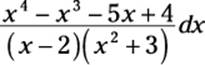
This looks like a good candidate for partial fractions, as I show you earlier in this chapter in “Case #2: Distinct quadratic factors.” But before you can express it as partial fractions, you need to determine whether it’s proper or improper. The degree of the numerator is 4 and (because the denominator is the product of a linear and a quadratic) the degree of the entire denominator is 3. Thus, this is an improper polynomial fraction (see “Distinguishing proper and improper rational expressions” earlier in this chapter). As a result, you can’t integrate by parts.

However, you can use polynomial division to turn this improper polynomial fraction into an expression that includes a proper polynomial fraction (I omit these steps here, but I show you how earlier in this chapter in “Recalling polynomial division.”):

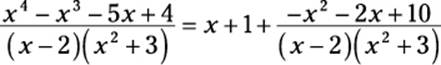
As you can see, the first two terms of this expression are simple to integrate (don’t forget about them!). To set up the remaining term for integration, use partial fractions:

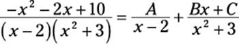
Get a common denominator on the right side of the equation:

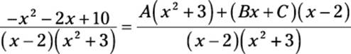
Now multiply both sides of the equation by this denominator:

–x² – 2x + 10 = A(x² + 3) + (Bx + C)(x – 2)

Notice that (x – 2) is a linear factor, so you can use the root of this factor to find the value of A. To find this value, let x = 2 and solve for A:

–(2²) – 2(2) + 10 = A(2² + 3) + (B2 + C)(2 – 2)

2 = 7A

Substitute this value into the equation:

At this point, to find the values of B and C, you need to split the equation into a system of two equations (as I show you earlier in “Working systematically with a system of equations”):

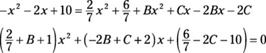
This splits into three equations:

–2B + C + 2 = 0

The first and the third equations show you that B = and C = . Now you can plug the values of A, B, and C back into the sum of partial fractions:

Make sure that you remember to add in the two terms (x + 1) that you left behind just after you finished your polynomial division:

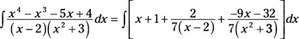
Thus, you can rewrite the original integral as the sum of five separate integrals:

You can solve the first two of these integrals by looking at them, and the next two by variable substitution (see Chapter 5). The last is done by using the following rule:

Here’s the solution so that you can work the last steps yourself: