Calculus For Dummies, 2nd Edition (2014)

Part V. Integration and Infinite Series

Chapter 15. Integration: It’s Backwards Differentiation

IN THIS CHAPTER

Using the area function

Getting familiar with the fundamental theorem of calculus

Finding antiderivatives

Figuring exact areas the easy way

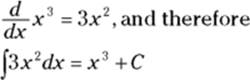
Chapter 14 shows you the hard way to calculate the area under a function using the formal definition of integration — the limit of a Riemann sum. In this chapter, I calculate areas the easy way, taking advantage of one of the most important and amazing discoveries in mathematics — that integration (finding areas) is just differentiation in reverse. That reverse process was a great discovery, and it’s based on some difficult ideas, but before we get to that, let’s talk about a related, straightforward reverse process, namely…

Antidifferentiation

The derivative of sin x is cos x, so the antiderivative of cos x is sin x; the derivative of is , so the antiderivative of is — you just go backwards. There’s a bit more to it, but that’s the basic idea. Later in this chapter, I show you how to find areas by using antiderivatives. This is much easier than finding areas with the Riemann sum technique.

Now consider and its derivative again. The derivative of is also , as is the derivative of . Any function of the form , where C is any number, has a derivative of . So, every such function is an antiderivative of .

Definition of the indefinite integral: The indefinite integral of a function , written as , is the family of all antiderivatives of the function. For example, because the derivative of is , the indefinite integral of is , and you write

You probably recognize this integration symbol, from the discussion of the definite integral in Chapter 14. The definite integral symbol, however, contains two little numbers like that tell you to compute the area under a function between those two numbers, called the limits of integration. The naked version of the symbol, indicates an indefinite integral or an antiderivative. This chapter is all about the intimate connection between these two symbols, these two ideas.

Figure 15-1 shows the family of antiderivatives of , namely . Note that this family of curves has an infinite number of curves. They go up and down forever and are infinitely dense. The vertical gap of 2 units between each curve in Figure 15-1 is just a visual aid.

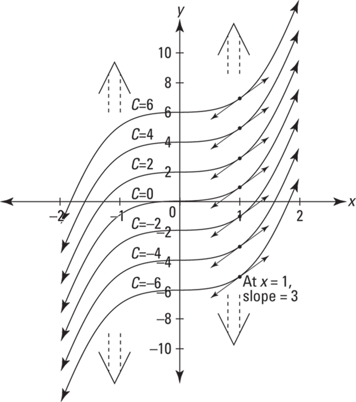
FIGURE 15-1: The family of curves All these functions have the same derivative,

Consider a few things about Figure 15-1. The top curve on the graph is ; the one below it is ; the bottom one . By the power rule, these three functions, as well as all the others in this family of functions, have a derivative of . Now, consider the slope of each of the curves where x equals 1 (see the tangent lines drawn on the curves). The derivative of each function is , so when x equals 1, the slope of each curve is , or 3. Thus, all these little tangent lines are parallel. Next, notice that all the functions in Figure 15-1 are identical except for being slid up or down (remember vertical shifts from Chapter 5?). Because they differ only by a vertical shift, the steepness at any x-value, like at , is the same for all the curves. This is the visual way to understand why each of these curves has the same derivative, and, thus, why each curve is an antiderivative of the same function.

Vocabulary, Voshmabulary: What Difference Does It Make?

In general, definitions and vocabulary are very important in mathematics, and it’s a good idea to use them correctly. But with the current topic, I’m going to be a bit lazy about precise terminology, and I hereby give you permission to do so as well.

If you’re a stickler, you should say that the indefinite integral of is and that is the family or set of all antiderivatives of (you don’t say that is the antiderivative), and you say that , for instance, is an antiderivative of . And on a test, you should definitely write . If you leave the C off, you’ll likely lose some points.

But, when discussing these matters, no one will care or be confused if you get tired of saying “+ C” after every indefinite integral and just say, for example, that the indefinite integral of is , and you can skip the indefiniteand just say that the integral of is . And instead of always talking about that family of functions business, you can just say that the antiderivative of is or that the antiderivative of is . Everyone will know what you mean. It may cost me my membership in the National Council of Teachers of Mathematics, but at least occasionally, I use this loose approach.

The Annoying Area Function

This is a tough one — gird your loins. Say you’ve got any old function, . Imagine that at some t-value, call it s, you draw a fixed vertical line. See Figure 15-2.

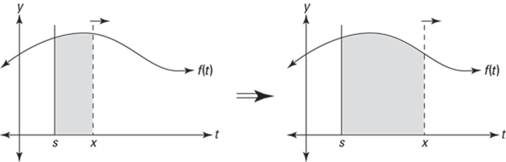
FIGURE 15-2: Area under f  between s and x is swept out by the moving line at x.

Then you take a moveable vertical line, starting at the same point, s (“s” is for starting point), and drag it to the right. As you drag the line, you sweep out a larger and larger area under the curve. This area is a function of x, the position of the moving line. In symbols, you write

Note that t is the input variable in instead of x because x is already taken — it’s the input variable in . The subscript f in indicates that is the area function for the particular curve f or . The dt is a little increment along the t-axis — actually an infinitesimally small increment.

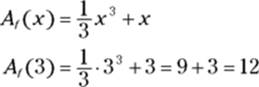
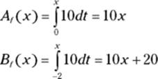
Here’s a simple example to make sure you’ve got a handle on how an area function works. By the way, don’t feel bad if you find this extremely hard to grasp — you’ve got lots of company. Say you’ve got the simple function, , that’s a horizontal line at . If you sweep out area beginning at , you get the following area function:

You can see that the area swept out from 3 to 4 is 10 because, in dragging the line from 3 to 4, you sweep out a rectangle with a width of 1 and a height of 10, which has an area of 1 times 10, or 10. See Figure 15-3.

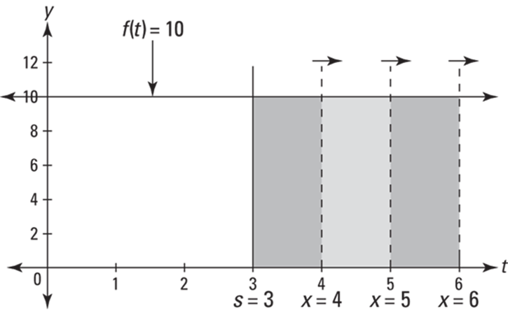
FIGURE 15-3: Area under between 3 and x is swept out by the moving vertical line at x.

So, , the area swept out as you hit 4, equals 10. equals 20 because when you drag the line to 5, you’ve swept out a rectangle with a width of 2 and height of 10, which has an area of 2 times 10, or 20. equals 30, and so on.

Now, imagine that you drag the line across at a rate of one unit per second. You start at , and you hit 4 at 1 second, 5 at 2 seconds, 6 at 3 seconds, and so on. How much area are you sweeping out per second? Ten square units per second because each second you sweep out another 1-by-10 rectangle. Notice — this is huge — that because the width of each rectangle you sweep out is 1, the area of each rectangle — which is given by height times width — is the same as its height because anything times 1 equals itself. You see why this is huge in a minute. (By the way, the real rate we care about here is not area swept out per second, but, rather, area swept out per unit change on the x-axis. I explain it in terms of per second because it’s easier to think about a sweeping-out-area rate this way. And since you’re dragging the line across at one x-axis unit per one second, both rates are the same. Take your pick.)

The derivative of an area function equals the rate of area being swept out. Okay, are you sitting down? You’ve reached another one of the big Ah ha! moments in the history of mathematics. Recall that a derivative is a rate. So, because the rate at which the previous area function grows is 10 square units per second, you can say its derivative equals 10. Thus, you can write

Again, this just tells you that with each 1 unit increase in x, (the area function) goes up 10. Now here’s the critical thing: Notice that this rate or derivative of 10 is the same as the height of the original function because as you go across 1 unit, you sweep out a rectangle that’s 1 by 10, which has an area of 10, the height of the function.

And the rate works out to 10 regardless of the width of the rectangle. Imagine that you drag the vertical line from to . At a rate of one unit per second, that’ll take you 1/1,000^th of a second, and you’ll sweep out a skinny rectangle with a width of 1/1,000, a height of 10, and thus an area of 10 times 1/1,000, or 1/100 square units. The rate of area being swept out would be, therefore, which equals 10 square units per second. So you see that with every small increment along the x-axis, the rate of area being swept out equals the function’s height.

This works for any function, not just horizontal lines. Look at the function and its area function that sweeps out area beginning at in Figure 15-4.

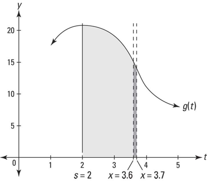
FIGURE 15-4: Area under between 2 and x is swept out by the moving vertical line at x.

Between and , grows by the area of that skinny, dark shaded “rectangle” with a width of 0.1 and a height of about 15. (As you can see, it’s not really a rectangle; it’s closer to a trapezoid, but it’s not that either because its tiny top is curving slightly. But, in the limit, as the width gets smaller and smaller, the skinny “rectangle” behaves precisely like a real rectangle.) So, to repeat, grows by the area of that dark “rectangle” which has an area extremely close to 0.1 times 15, or 1.5. That area is swept out in 0.1 seconds, so the rate of area being swept out is , or 15 square units per second, the height of the function. This idea is so important that it deserves an icon.

The sweeping out area rate equals the height. The rate of area being swept out under a curve by an area function at a given x-value is equal to the height of the curve at that x-value.

The Power and the Glory of the Fundamental Theorem of Calculus

Sound the trumpets! Now that you’ve seen the connection between the rate of growth of an area function and the height of the given curve, you’re ready for the fundamental theorem of calculus — what some say is one of the most important theorems in the history of mathematics.

The fundamental theorem of calculus: Given an area function that sweeps out area under ,

the rate at which area is being swept out is equal to the height of the original function. So, because the rate is the derivative, the derivative of the area function equals the original function:

Because you can also write the above equation as follows:

Break out the smelling salts.

Now, because the derivative of is , is by definition an antiderivative of . Check out how this works by returning to the simple function from the previous section, , and its area function, .

According to the fundamental theorem, . Thus must be an antiderivative of 10; in other words, is a function whose derivative is 10. Because any function of the form , where C is a number, has a derivative of 10, the antiderivative of 10 is . The particular number C depends on your choice of s, the point where you start sweeping out area. For a particular choice of s, the area function will be the one function (out of all the functions in the family of curves ) that crosses the x-axis at s. To figure out C, set the antiderivative equal to zero, plug the value of s into x, and solve for C.

For this function with an antiderivative of , if you start sweeping out area at, say, , then , so , and thus, , or just 10x. (Note that C does not necessarily equal s. In fact, it usually doesn’t [especially when ]. When , C often also equals 0, but not for all functions.)

Figure 15-5 shows why is the correct area function if you start sweeping out area at zero. In the top graph in the figure, the area under the curve from 0 to 3 is 30, and that’s given by . And you can see that the area from 0 to 5 is 50, which agrees with the fact that .

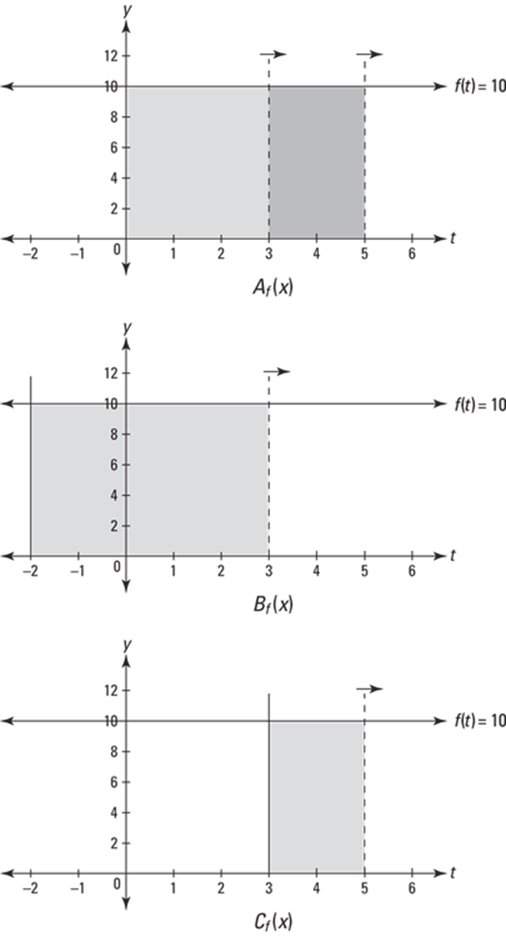
FIGURE 15-5: Three area functions for

If instead you start sweeping out area at and define a new area function, , then , so C equals 20 and is thus . This area function is 20 more than , which starts at , because if you start at , you’ve already swept out an area of 20 by the time you get to zero. Figure 15-5 shows why is 20 more than .

And if you start sweeping out area at , , so and the area function is . This function is 30 less than because with , you lose the 3-by-10 rectangle between 0 and 3 that has (see the bottom graph in Figure 15-5).

An area function is an antiderivative. The area swept out under the horizontal line from some number s to x, is given by an antiderivative of 10, namely where the value of C depends on where you start sweeping out area.

Now let’s look at graphs of , , and . (Note that Figure 15-5 doesn’t show the graphs of , , and . You see three graphs of the horizontal line function, ; and you see the areas swept out under by , , and , but you don’t actually see the graphs of these three area functions.) Check out Figure 15-6.

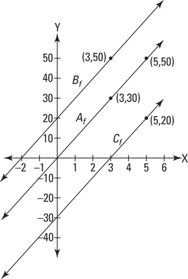
FIGURE 15-6: The actual graphs of

Figure 15-6 shows the graphs of the equations of , , and which we worked out before: , , and . (As you can see, all three are simple, lines.) The y-values of these three functions give you the areas swept out under that you see in Figure 15-5. Note that the three x-intercepts you see in Figure 15-6 are the three x-values in Figure 15-5 where sweeping out area begins.

We worked out above that and that . You can see those areas of 30 and 50 in the top graph of Figure 15-5. In Figure 15-6, you see these results on at the points and . You also saw in Figure 15-5 that was 20 more than ; you see that result in Figure 15-6 where on is 20 higher than (3, 30) on . Finally, you saw in Figure 15-5 that is 30 less than . Figure 15-6 shows that in a different way: at any x-value, the line is 30 units below the line.

A few observations. You already know from the fundamental theorem that (and the same for and ). That was explained above in terms of rates: For , , and , the rate of area being swept out under equals 10. Figure 15-6 also shows that (and the same for and ), but here you see the derivative as a slope. The slopes, of course, of all three lines equal 10. Finally, note that — like you saw in Figure 15-1 — the three lines in Figure 15-6 differ from each other only by a vertical translation. These three lines (and the infinity of all other vertically translated lines) are all members of the class of functions, , the family of antiderivatives of .

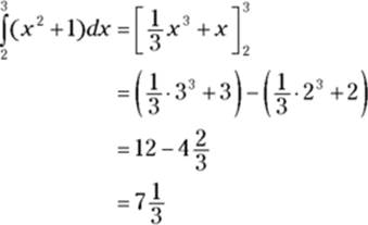
For the next example, look again at the parabola , our friend from Chapter 14 which we analyzed in terms of the sum of the areas of rectangles (Riemann sums). Flip back to Figure 14-4, and check out the shaded region under . Now you can finally compute the exact area of the shaded region the easy way.

The area function for sweeping out area under is . By the fundamental theorem, , and so is an antiderivative of . Any function of the form has a derivative of (try it), so that’s the antiderivative. For Figure 14-6, you want to sweep out area beginning at 0, so . Set the antiderivative equal to zero, plug the value of s into x, and solve for C: , so , and thus

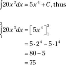
The area swept out from 0 to 3 — which we did the hard way in Chapter 14 by computing the limit of a Riemann sum — is simply :

Piece o’ cake. That was much less work than doing it the hard way.

And after you know that the area function that starts at zero, it’s a snap to figure the area of other sections under the parabola that don’t start at zero. Say, for example, you want the area under the parabola between 2 and 3. You can compute that area by subtracting the area between 0 and 2 from the area between 0 and 3. You just figured the area between 0 and 3 — that’s 12. And the area between 0 and 2 is . So the area between 2 and 3 is , or . This subtraction method brings us to the next topic — the second version of the fundamental theorem.

The Fundamental Theorem of Calculus: Take Two

Now we finally arrive at the super-duper shortcut integration theorem that you’ll use for the rest of your natural born days — or at least till the end of your stint with calculus. This shortcut method is all you need for the integration word problems in Chapters 17 and 18.

The fundamental theorem of calculus (second version or shortcut version): Let F be any antiderivative of the function f; then

This theorem gives you the super shortcut for computing a definite integral like , the area under the parabola between 2 and 3. As I show in the previous section, you can get this area by subtracting the area between 0 and 2 from the area between 0 and 3, but to do that you need to know that the particular area function sweeping out area beginning at zero, , is (with a C value of zero).

The beauty of the shortcut theorem is that you don’t have to even use an area function like . You just find any antiderivative, , of your function, and do the subtraction, . The simplest antiderivative to use is the one where . So here’s how you use the theorem to find the area under our parabola from 2 to 3. is an antiderivative of . Then the theorem gives you:

Granted, this is the same computation I did in the previous section using the area function with , but that’s only because for the function, when s is zero, C is also zero. It’s sort of a coincidence, and it’s not true for all functions. But regardless of the function, the shortcut works, and you don’t have to worry about area functions or s or C. All you do is .

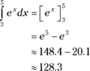
Here’s another example: What’s the area under between and   ? The derivative of is , so is an antiderivative of , and thus

What could be simpler?

Areas above the curve and below the x-axis count as negative areas. Before going on, I’d be remiss if I didn’t touch on negative areas (this is virtually the same caution made at the very end of Chapter 14). Note that with the two examples above, the parabola, , and the exponential function, the areas we’re computing are under the curves and above the x-axis. These areas count as ordinary, positive areas. But, if a function goes below the x-axis, areas above the curve and below the x-axis count as negative areas. This is the case whether you’re using an area function, the first version of the fundamental theorem of calculus, or the shortcut version. Don’t worry about this for now. You see how this works in Chapter 17.

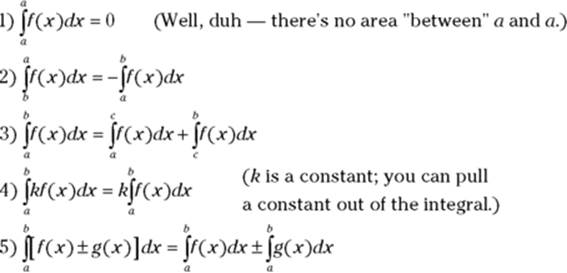
Okay, so now you’ve got the super shortcut for computing the area under a curve. And if one big shortcut wasn’t enough to make your day, Table 15-1 lists some rules about definite integrals that can make your life much easier.

TABLE 15-1 Five Easy Rules for Definite Integrals

Now that I’ve given you the shortcut version of the fundamental theorem, that doesn’t mean you’re off the hook. Below are three different ways to understand why the theorem works. This is difficult stuff — brace yourself.

Alternatively, you can skip these explanations if all you want to know is how to compute an area: forget about C and just subtract from . I include these explanations because I suspect you’re dying to learn extra math just for the love of learning — right? Other books just give you the rules; I explain why they work and the underlying principles — that’s why they pay me the big bucks.

Actually, in all seriousness, you should read at least some of this material. The fundamental theorem of calculus is one of the most important theorems in all of mathematics, so you ought to spend some time trying hard to understand what it’s all about. It’s worth the effort. Of the three explanations, the first is the easiest. But if you only want to read one or two of the three, I’d read just the third, or the second and the third. Or, you could begin with the figures accompanying the three explanations, because the figures really show you what’s going on. Finally, if you can’t digest all of this in one sitting — no worries — you can revisit it later.

Why the theorem works: Area functions explanation

One way to understand the shortcut version of the fundamental theorem is by looking at area functions. As you can see in Figure 15-7, the dark-shaded area between a and b can be figured by starting with the area between s and b, then cutting away (subtracting) the area between s and a. And it doesn’t matter whether you use 0 as the left edge of the areas or any other value of s. Do you see that you’d get the same result whether you use the graph on the left or the graph on the right?

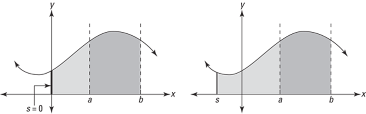
FIGURE 15-7: Figuring the area between a and b with two different area functions.

Take a look at (see Figure 15-8). Say you want the area between 5 and 8 under the horizontal line , and you are forced to use calculus.

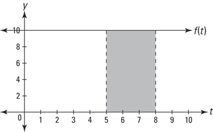
FIGURE 15-8: The shaded area equals 30 — well, duh, it’s a 3-by-10 rectangle.

Look back at two of the area functions for in Figure 15-5: starting at 0 (in which ) and starting at :

If you use to compute the area between 5 and 8 in Figure 15-8, you get the following:

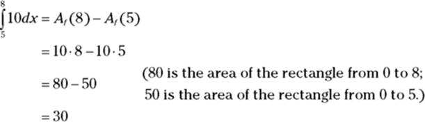
If, on the other hand, you use to compute the same area, you get the same result:

Notice that the two 20s in the second line from the bottom cancel. Recall that all antiderivatives of are of the form . Regardless of the value of C, it cancels out as in this example. Thus, you can use any antiderivative with any value of C. For convenience, everyone just uses the antiderivative with so that you don’t mess with C at all. And the choice of s (the point where the area function begins) is irrelevant. So when you’re using the shortcut version of the fundamental theorem, and computing an area with , you’re sort of using a mystery area function with a C value of zero and an unknown starting point, s. Get it?

Why the theorem works: The integration-differentiation connection

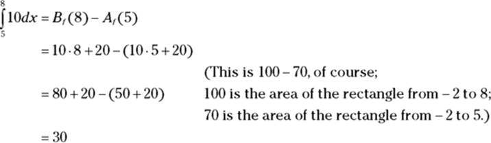
The next explanation of the shortcut version of the fundamental theorem involves the yin/yang relationship between differentiation and integration. Check out Figure 15-9.

FIGURE 15-9: The essence of differentiation and integration in a single figure! It’s a yin/yang thing.

The figure shows a function, , and its derivative, . Look carefully at the numbers 4, 6, and 8 on both graphs. The connection between 4, 6, and 8 on the graph of f — which are the amounts of risebetween consecutive points on the curve — and 4, 6, and 8 on the graph of — which are the areas of the trapezoids under — shows the intimate relationship between integration and differentiation. Figure 15-9 is a picture worth a thousand symbols and equations, encapsulating the essence of integration in a single snapshot. It shows how the shortcut version of the fundamental theorem works because it shows that the area under between 1 and 4 equals the total rise on between and , in other words that

Note that I’ve called the two functions in Figure 15-9 and in the above equation f and to emphasize that is the derivative of . I could have instead referred to as F and referred to as f which would emphasize that is an antiderivative of . In that case you would write the above area equation in the standard way,

Either way, the meaning’s the same. I use the derivative version to point out how finding area is differentiation in reverse. Going from left to right in Figure 15-9 is differentiation: The slopes of f correspond to heights on . Going from right to left is integration: Areas under correspond to the change in height between two points on f.

Okay, here’s how it works. Imagine you’re going up along f from to . Every point along the way has a certain steepness, a slope. This slope is plotted as the y-coordinate, or height, on the graph of . The fact that goes up from to tells you that the slope of f goes up from 3 to 5 as you travel between and . This all follows from basic differentiation.

Now, as you go along f from to , the slope is constantly changing. But it turns out that because you go up a total rise of 4 as you run across 1, the average of all the slopes on f between and is , or 4. Because each of these slopes is plotted as a y-coordinate or height on , it follows that the average height of between and is also 4. Thus, between two given points, average slope on f equals average height on .

Hold on, you’re almost there. Slope equals , so when the run is 1, the slope equals the rise. For example, from to on f, the curve rises up 4 and the average slope between those points is also 4. Thus, between any two points on f whose x-coordinates differ by 1, the average slope is the rise.

The area of a trapezoid like the ones on the right in Figure 15-9 equals its width times its average height. (This is true of any other similar shape that has a bottom like a rectangle; the top can be any crooked line or funky curve you like.) So, because the width of each trapezoid is 1, and because anything times 1 is itself, the average height of each trapezoid under is its area; for instance, the area of that first trapezoid is 4 and its average height is also 4.

Are you ready for the grand finale? Here’s the whole argument in a nutshell. On f, ; going from f to , ; on , . So that gives you , and thus, finally, . And that’s what the second version of the fundamental theorem says:

These ideas are unavoidably difficult. You may have to read it two or three times for it to really sink in.

Notice that it makes no difference to the relationship between slope and area if you use any other function of the form instead of . Any parabola like or is exactly the same shape as ; it’s just been slid up or down vertically. Any such parabola rises up between and in precisely the same way as the parabola in Figure 15-9. From 1 to 2 these parabolas go over 1, up 4. From 2 to 3 they go over 1, up 6, and so on. This is why any antiderivative can be used to find area. The total area under between 1 to 4, namely 18, corresponds to the total rise on any of these parabolas from 1 to 4, namely , or 18.

At the risk of beating a dead horse, I’ve got a third explanation of the fundamental theorem for you. You might prefer it to the first two because it’s less abstract — it’s connected to simple, commonsense ideas encountered in our day-to-day world. This explanation has a lot in common with the previous one, but the ideas are presented from a different angle.

Why the theorem works: A connection to — egad! — statistics

Don’t let the title of this section put you off. I realize that many readers of this calculus book may not have studied statistics. No worries; the statistics connection I explain below involves a very simple thing covered in statistics courses, but you don’t need to know any statistics at all to understand this idea. The simple idea is the relationship between a frequency distribution graph and a cumulative frequency distribution graph (you may have run across such graphs in a newspaper or magazine). Consider Figure 15-10.

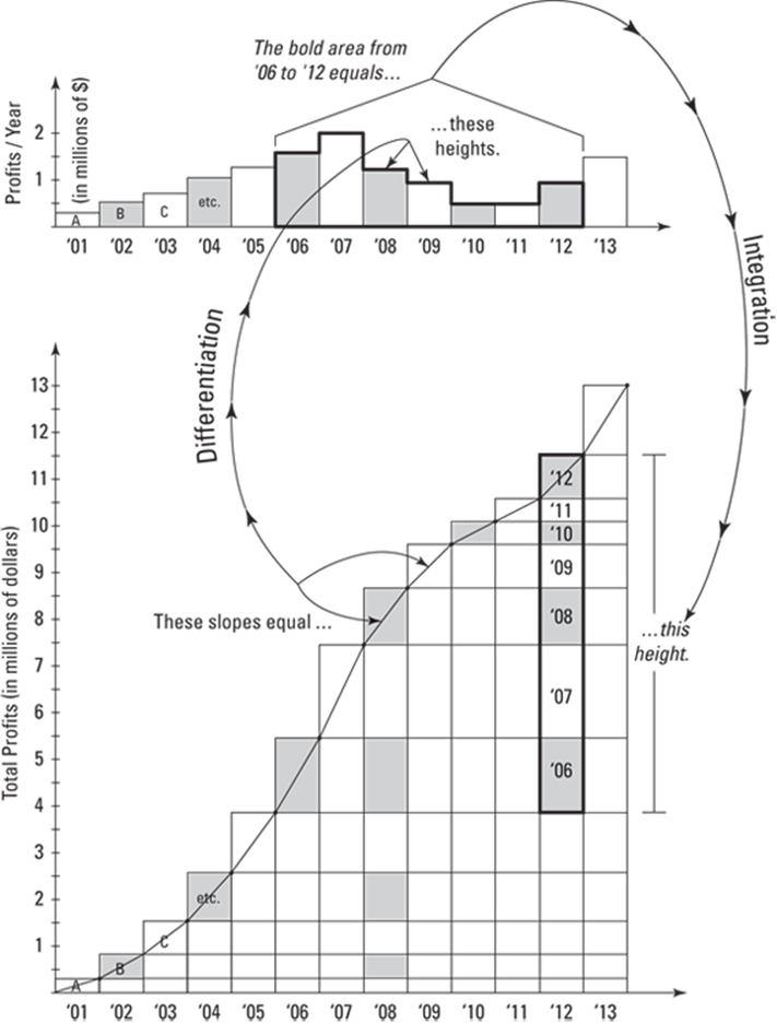
FIGURE 15-10: A frequency distribution histogram (above) and a cumulative frequency distribution histogram (below) for the annual profits of Widgets-R-Us show the connection between differentiation and integration.

The upper graph in the figure shows a frequency distribution histogram of the annual profits of Widgets-R-Us from January 1, 2001 through December 31, 2013. The rectangle marked ’07, for example, shows that the company’s profit for 2007 was $2,000,000 (their best year during the period 2001–2013).

The lower graph in the figure is a cumulative frequency distribution histogram for the same data used for the upper graph. The difference is simply that in the cumulative graph, the height of each column shows the total profits earned since 1/1/2001. Look at the ’02 column in the lower graph and the ’01 and ’02 rectangles in the upper graph, for example. You can see that the ’02 column shows the ’02 rectangle sitting on top of the ’01 rectangle which gives that ’02 column a height equal to the total of the profits from ’01 and ’02. Got it? As you go to the right on the cumulative graph, the height of each successive column simply grows by the amount of profits earned in the corresponding single year shown in the upper graph.

Okay. So here’s the calculus connection. (Bear with me; it takes a while to walk through all this.) Look at the top rectangle of the ’08 column on the cumulative graph (let’s call that graph C for short). At that point on C, you runacross 1 year and rise up $1,250,000, the ’08 profit you see on the frequency distribution graph (F for short). , so, since the run equals 1, the slope equals 1,250,000/1, or just 1,250,000, which is, of course, the same as the rise. Thus, the slope on C (at ’08 or any other year) can be read as a height on F for the corresponding year. (Make sure you see how this works.) Since the heights (or function values) on F are the slopes of C, F is the derivative of C. In short, F, the derivative, tells us about the slope of C.

The next idea is that since F is the derivative of C, C, by definition, is the antiderivative of F (for example, C might equal and F would equal ). Now, what does C, the antiderivative of F, tell us about F ? Imagine dragging a vertical line from left to right over F. As you sweep over the rectangles on F — year by year — the total profit you’re sweeping over is shown climbing up along C.

Look at the ’01 through ’08 rectangles on F. You can see those same rectangles climbing up stair-step fashion along C (see the rectangles labeled A, B, C, etc. on both graphs). The heights of the rectangles from F keep adding up on C as you climb up the stair-step shape. And I’ve shown how the same ’01 through ’08 rectangles that lie along the stair-step top of C can also be seen in a vertical stack at year ’08 on C. I’ve drawn the cumulative graph his way so it’s even more obvious how the heights of the rectangles add up. (Note: Most cumulative histograms are not drawn this way.)

Each rectangle on F has a base of 1 year, so, since , the area of each rectangle equals its height. So, as you stack up rectangles on C, you’re adding up the areas of those rectangles from F. For example, the height of the ’01 through ’08 stack of rectangles on C ($8.5 million) equals the total area of the ’01 through ’08 rectangles on F. And, therefore, the heights or function values of C — which is the antiderivative of F — give you the area under the top edge of F. That’s how integration works.

Okay, we’re just about done. Now let’s go through how these two graphs explain the shortcut version of the fundamental theorem of calculus and the relationship between differentiation and integration. Look at the ’06 through ’12 rectangles on F (with the bold border). You can see those same rectangles in the bold portion of the ’12 column of C. The height of that bold stack, which shows the total profits made during those 7 years, $7.75 million, equals the total area of the 7 rectangles in F. And to get the height of that stack on C, you simply subtract the height of the stack’s bottom edge from the height of its upper edge. That’s really all the shortcut version of the fundamental theorem says: The area under any portion of a function (like F) is given by the change in height on the function’s antiderivative (like C).

In a nutshell (keep looking at those rectangles with the bold border in both graphs), the slopes of the rectangles on C appear as heights on F. That’s differentiation. Reversing direction, you see integration: the change in heightson C shows the area under F. Voilà: Differentiation and integration are two sides of the same coin.

(Note: Mathematical purists may object to this explanation of the fundamental theorem because it involves discrete graphs (for example, the fact that the cumulative distribution histogram in Figure 15-10 goes up at one-year increments), whereas calculus is the study of smooth, continuously changing graphs (the calculus version of the cumulative distribution histogram would be a smooth curve that would show the total profits growing every millisecond — actually, in theory, every infinitesimal fraction of a second). Okay — objection noted — but the fact is that the explanation here does accurately show how integration and differentiation are related and does correctly show how the shortcut version of the fundamental theorem works. All that’s needed to turn Figure 15-10 and the accompanying explanation into standard calculus is to take everything to the limit, making the profit interval shorter and shorter and shorter: from a year to a month to a day, etc., etc. In the limit, the discrete graphs in Figure 15-10 would meld into the type of smooth graphs used in calculus. But the ideas wouldn’t change. The ideas would be exactly as explained here. This is very similar to what you saw in Chapter 14 where you first approximated the area under a curve by adding up the areas of rectangles and then were able to compute the exact area by using the limit process to narrow the widths of the rectangles till their widths became infinitesimal.)

Well, there you have it — actual explanations of why the shortcut version of the fundamental theorem works and why finding area is differentiation in reverse. If you understand only half of what I’ve just written, you’re way ahead of most students of calculus. The good news is that you probably won’t be tested on this theoretical stuff. Now let’s come back down to earth.

Finding Antiderivatives: Three Basic Techniques

I’ve been talking a lot about antiderivatives, but just how do you find them? In this section, I give you three easy techniques. Then in Chapter 16, I give you four advanced techniques. By the way, you will be tested on this stuff.

Reverse rules for antiderivatives

The easiest antiderivative rules are the ones that are the reverse of derivative rules you already know. (You can brush up on derivative rules in Chapter 10 if you need to.) These are automatic, one-step antiderivatives with the exception of the reverse power rule, which is only slightly harder.

No-brainer reverse rules

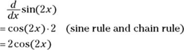
You know that the derivative of sinx is cosx, so reversing that tells you that an antiderivative of cosx is sinx. What could be simpler? But don’t forget that all functions of the form are antiderivatives of cosx. In symbols, you write

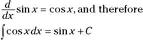
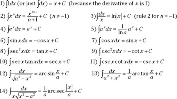
Table 15-2 lists the reverse rules for antiderivatives.

TABLE 15-2 Basic Antiderivative Formulas

The slightly more difficult reverse power rule

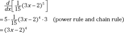
By the power rule for differentiation, you know that

Here’s the simple method for reversing the power rule. Use for your function. Recall that the power rule says to

1. Bring the power in front where it will multiply the rest of the derivative.

2. Reduce the power by one and simplify.

Thus, .

To reverse this process, you reverse the order of the two steps and reverse the math within each step. Here’s how that works for the above problem:

1. Increase the power by one.

The 3 becomes a 4.

2. Divide by the new power and simplify.

And thus you write .

The reverse power rule does not work for a power of negative one. The reverse power rule works for all powers (including negative and decimal powers) except for a power of negative one. Instead of using the reverse power rule, you should just memorize that the antiderivative of is (rule 3 in Table 15-2).

Test your antiderivatives by differentiating them. Especially when you’re new to antidifferentiation, it’s a good idea to test your antiderivatives by differentiating them — you can ignore the C. If you get back to your original function, you know your antiderivative is correct.

With the antiderivative you just found and the shortcut version of the fundamental theorem, you can determine the area under between, say, 1 and 2:

Guessing and checking

The guess-and-check method works when the integrand (that’s the expression after the integral symbol not counting the dx, and it’s the thing you want to antidifferentiate) is close to a function that you know the reverse rule for. For example, say you want the antiderivative of . Well, you know that the derivative of sine is cosine. Reversing that tells you that the antiderivative of cosine is sine. So you might think that the antiderivative of is . That’s your guess. Now check it by differentiating it to see if you get the original function, :

This result is very close to the original function, except for that extra coefficient of 2. In other words, the answer is 2 times as much as what you want. Because you want a result that’s half of this, just try an antiderivative that’s half of your first guess: So your new guess is . Check this second guess by differentiating it, and you get the desired result.

Here’s another example. What’s the antiderivative of    ?

1. Guess the antiderivative.

This looks sort of like a power rule problem, so try the reverse power rule. The antiderivative of is by the reverse power rule, so your guess is .

2. Check your guess by differentiating it.

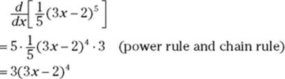
3. Tweak your first guess.

Your result, is three times too much, so make your second guess a third of your first guess — that’s , or .

4. Check your second guess by differentiating it.

This checks. You’re done. The antiderivative of is .

The two previous examples show that guess and check works well when the function you want to antidifferentiate has an argument like 3x or (where x is raised to the first power) instead of a plain old x. (Recall that in a function like , the 5x is called the argument.) In this case, all you have to do is tweak your guess by the reciprocal of the coefficient of x: the 3 in , for example (the 2 in has no effect on your answer). In fact, for these easy problems, you don’t really have to do any guessing and checking. You can immediately see how to tweak your guess. It becomes sort of a one-step process. If the function’s argument is more complicated than — like the in — you have to try the next method, substitution.

The substitution method

If you look back at the examples of the guess and check method in the previous section, you can see why the first guess in each case didn’t work. When you differentiate the guess, the chain rule produces an extra constant: 2 in the first example, 3 in the second. You then tweak the guesses with and to compensate for the extra constant.

Now say you want the antiderivative of and you guess that it is . Watch what happens when you differentiate to check it:

Here the chain rule produces an extra 2x — because the derivative of is 2x — but if you try to compensate for this by attaching a to your guess, it won’t work. Try it.

So, guessing and checking doesn’t work for antidifferentiating — actually no method works for this simple-looking integrand (not all functions have antiderivatives) — but your admirable attempt at differentiation here reveals a new class of functions that you can antidifferentiate. Because the derivative of is , the antiderivative of must be . This function, , is the type of function you can antidifferentiate with the substitution method.

Keep your eyes peeled for the derivative of the function’s argument. The substitution method works when the integrand contains a function and the derivative of the function’s argument — in other words, when it contains that extra thing produced by the chain rule — or something just like it except for a constant. And the integrand must not contain any other extra stuff.

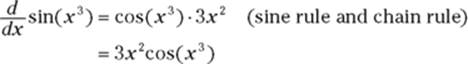
The derivative of is ·   by the rule and the chain rule. So, the antiderivative of is . And if you were asked to find the antiderivative of , you would know that the substitution method would work because this expression contains , which is the derivative of the argument of , namely .

By now, you’re probably wondering why this is called the substitution method. I show you why in the step-by-step method below. But first, I want to point out that you don’t always have to use the step-by-step method. Assuming you understand why the antiderivative of is , you may encounter problems where you can just see the antiderivative without doing any work. But whether or not you can just see the answers to problems like that one, the substitution method is a good technique to learn because, for one thing, it has many uses in calculus and other areas of mathematics, and for another, your teacher may require that you know it and use it. Okay, so here’s how to find with substitution:

1. Set u equal to the argument of the main function.

The argument of is , so you set u equal to .

2. Take the derivative of u with respect to x.

3. Solve for dx.

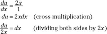
4. Make the substitutions.

In , u takes the place of and takes the place of dx. So now you’ve got . The two 2xs cancel, giving you .

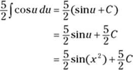
5. Antidifferentiate using the simple reverse rule.

6. Substitute back in for u, coming full circle.

u equals , so goes in for the u:

That’s it. So .

If the original problem had been instead of , you follow the same steps except that in Step 4, after making the substitution, you arrive at . The xs still cancel — that’s the important thing — but after canceling you get , which has that extra in it. No worries. Just pull the through the giving you . Now you finish this problem just as you did in Steps 5 and 6, except for the extra :

Because C is any old constant, is still any old constant, so you can get rid of the in front of the C. That may seem somewhat (grossly?) unmathematical, but it’s right. Thus, your final answer is . You should check this by differentiating it.

Here are a few examples of antiderivatives you can do with the substitution method so you can learn how to spot them:

· 

The derivative of is , but you don’t have to pay any attention to the 3 in or the 4 in the integrand. Because the integrand contains and no other extra stuff, substitution works. Try it.

· 

The integrand contains a function, , and the derivative of its argument (tanx) — which is . Because the integrand doesn’t contain any other extra stuff (except for the 10, which doesn’t matter), substitution works. Do it.

· 

Because the integrand contains the derivative of namely and no other stuff except for the , substitution works. Go for it.

You can do the three problems just listed with a method that combines substitution and guess-and-check (as long as your teacher doesn’t insist that you show the six-step substitution solution). Try using this combo method to antidifferentiate the first example, . First, you confirm that the integral fits the pattern for substitution — it does, as pointed out in the first item on the checklist. This confirmation is the only part substitution plays in the combo method. Now you finish the problem with the guess-and-check method:

1. Make your guess.

The antiderivative of cosine is sine, so a good guess for the antiderivative of is .

2. Check your guess by differentiating it.

3. Tweak your guess.

Your result from Step 2, is of what you want, , so make your guess bigger (note that is the reciprocal of ). Your second guess is thus .

4. Check this second guess by differentiating it.

Oh, heck, skip this — your answer’s got to work.

Finding Area with Substitution Problems

You can use the shortcut version of the fundamental theorem to calculate the area under a function that you integrate with the substitution method. You can do this in two ways. In the previous section, I use substitution, setting uequal to , to find the antiderivative of :

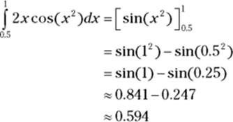
If you want the area under this curve from, say, 0.5 to 1, the fundamental theorem does the trick:

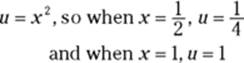
Another method, which amounts to the same thing, is to change the limits of integration and do the whole problem in terms of u. Refer back to the six-step solution in the section “The substitution method.” What follows is very similar, except that this time you’re doing definite integration rather than indefinite integration. Again, you want the area given by :

1. Set u equal to .

2. Take the derivative of u with respect to x.

3. Solve for dx.

4. Determine the new limits of integration.

5. Make the substitutions, including the new limits of integration, and cancel the two 2xs.

(In this problem, only one of the limits is new because when .)

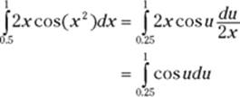
6. Use the antiderivative and the fundamental theorem to get the desired area without making the switch back to .

It’s a case of six of one, half a dozen of another with the two methods; they require about the same amount of work. So you can take your pick — however, most teachers and textbooks emphasize the second method, so you probably should learn it.