The Calculus Primer (2011)
Part XI. Expansion of Functions
Chapter 42. EXPANSION OF FUNCTIONS
11—13. Transforming a Function into a Power Series. It will be recalled from algebra that a function of the type (1 + x)k can be transformed into a series of terms which are powers of x. Thus if k is a positive integer, a finite series is obtained—the familiar binomial expansion of (k + 1) terms:
![]()
If, on the other hand, k is a negative integer or a fraction, the use of the binomial expansion leads to an infinite series, but not of the same type as (1), since x appears with negative or fractional exponents. By actual division to as many terms as desired, we obtain, for example:
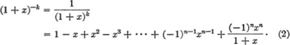
By this method of expansion there will always be a remainder,
![]()
this remainder will vanish only if R → 0 as n → ∞. The only condition under which R → 0 as n → ∞ is when |x| < 1. Hence series (2) can be used to find the approximate value of a function of the form (1 + x)−k only for values of xsuch that − 1 < x < 1; in this case, R → 0, and the series can be shown to be convergent for −1 < x < 1; the greater the number of terms taken, the closer the approximation will be.
No analogous method is available for the convenient expansion of (1 + x)k when k is a fraction.
11—14. Maclaurin’s Series. In order to arrive at a more general method of expanding a function into a power series, let us assume that, for a given function, f(x), there exists a power series equivalent to the function in question, and that this series has the form
f(x) = a0 + a1x + a2x2 + … + an−1xn−1 + … . (1)
To determine the value of the coefficients (the a’s) in (1), we may proceed as follows. Let f(x) = 0; then f(0) = a0. Let us assume that derivatives of all orders exist for f(x) at x = 0; let us also assume that f(x) can be differentiated term by term indefinitely often. To be sure, not all functions meet these requirements, but many functions do, and the present discussion is limited to such functions. Then, by differentiation, we have:
f′(x) = a1 + 2a2x + 3a3x2 + 4a4x3 + … ; f′(0) = 1·a1.
f″(x) = 2a2 + 3·2a3x + 4·3a4x2 + … ; f″(0) = 2·1a2.
f′″(x) = 3·2a3 + 4·3·2a4x + ... ; f′″(0) = 3·2·la3.
fn−1(x) = (n − 1)! an−1 + n!anx + … ; fn−1(0) = (n − 1)! an−1.
Substituting these values for the coefficients a0, a1, a2, … in equation (1), we obtain:
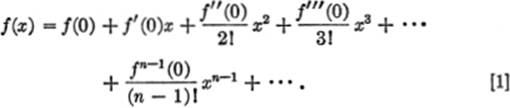
The expansion of f(x) given in [1] is known as Maclaurin’s series. When a function has been expanded in this way in a Maclaurin’s series, it is necessary (1) to bear in mind the assumptions made above, and (2) to determine the interval of convergence of the series.
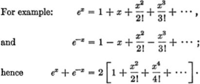
EXAMPLE 1. Expand in a Maclaurin’s series the function f(x) = ex.
Solution.
f(x) = ex f(0) = 1
f′(x) = ex f′(0) = 1
f′″(x) = ex f″(0) = 1
……… ………
Hence
![]()
Since ![]()
the series is convergent for all values of x.
EXAMPLE 2. Expand log (1 + x) in a Maclaurin’s series.
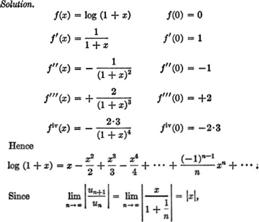
therefore the series is convergent for |x| < 1, or for — 1 < x < 1. To test the end points, we note that when x = +1, the series is also convergent; but when x = − 1, the series becomes, in effect, equivalent to the harmonic series, which is divergent.
11—15. The Binomial Expansion. In a similar manner, we can investigate, by using the Maclaurin’s series, the expansion of (1 + x)m. Thus,
f(x) = (1 + x)m f(0) = 1
f′(x) = m(1 + x)m−1 f′(0)= m
f″(x) = m(m − 1)(1 + x)m−2 f″(0) = m(m − 1)
……………………… ………………
Hence:
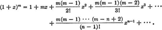
In other words, the familiar binomial theorem of algebra is valid not only when m is a positive integer, but also, for certain values of x, when m is a negative integer or a fraction. Applying the ratio test, we have:
![]()
which, when simplified, becomes
![]()
Hence, ![]() therefore the series is convergent for |x| < 1, or for − 1 < x < 1. Consequently the binomial expansion is valid for any value of m for values of x between − 1 and +1. Whether it is valid for the values ±1, the end points of the interval of convergence, depends upon the particular value of m; a discussion of this problem is beyond the scope of this book.
therefore the series is convergent for |x| < 1, or for − 1 < x < 1. Consequently the binomial expansion is valid for any value of m for values of x between − 1 and +1. Whether it is valid for the values ±1, the end points of the interval of convergence, depends upon the particular value of m; a discussion of this problem is beyond the scope of this book.
11—16. The Exponential Series. Let us consider the expansion of ex once more. In §11—14, Example 1, we learned that
![]()
Putting x = 1 in both sides of (1), we have:
![]()
We may evaluate numerically as follows:
1st term= 1.00000
2nd term = 1.00000
3rd term= .50000
4th term= .16667 …(by dividing 3rd term by 3)
5th term= .04167 …(by dividing 4th term by 4)
6th term= .00833 …(by dividing 5th term by 5)
7th term= .00139 …(by dividing 6th term by 6)
8th term= .00019 …(by dividing 7th term by 7)
2.71825 ...
Hence, the value of e, which may also be defined as
![]()
is equal to 2.7183, correct to four decimal places. This value is of considerable importance in applied mathematics; to ten decimal places, e = 2.71828 18285.
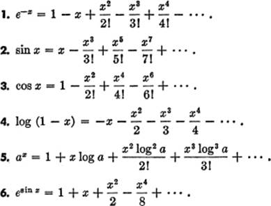
EXERCISE 11—5
Verify each of the following expansions; determine for what values of the variable they are convergent:
11—17. Taylor’s Series. It is often useful to develop a function as a power series in terms of ascending powers of (x − a), where a is some given constant. This leads to a series of the form
f(x) = c0 + c1(x − a) + c2(x − a)2 +
+ c3(x − a)3 + … + cn−1(x − a)n−1 + … .
Now, making the same assumptions with respect to this series as were made in §11—14, and following the same method of reasoning to determine the coefficients c0, c1, c2, … cn, we obtain the series
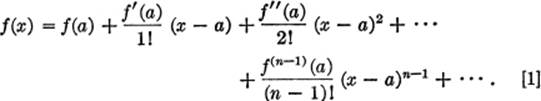
This series is known as Taylor’s series. It is a more general form of Maclaurin’s series; in other words, Maclaurin’s series is a special case of Taylor’s series, obtained by putting a = 0 in [1] above.
It should be pointed out that Maclaurin’s series is useful in computing the value of f(x) when x has values in the neighborhood of zero, for it is then that the series converges with greatest rapidity; for the same reason, Taylor’s series is most useful for computing the value of f(x) when x has values near to a, whatever the constant value of a may be.
11—18. Other Forms of Taylor’s Series. A function of the sum of two quantities, for example, f(x + h), may be expanded in powers of one of those quantities. This may be deduced from equation [1] above by taking a = h,and substituting (x + h) for x; thus
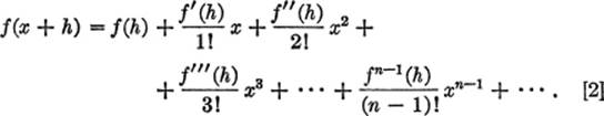
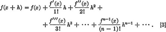
Finally, if we interchange x and h in equation [2], observing that f(h + x) ≡ f(x + h), we obtain an alternative form of Taylor’s series for f(x + h) in powers of the number h; thus
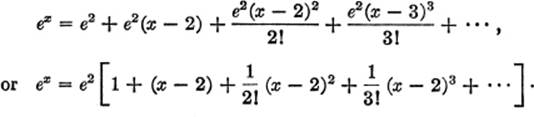
EXAMPLE 1. Expand ex in terms of powers of (x − 2).
Solution. Here f(x) = ex; x − a = x − 2, or a = 2.
Hence f′(x) = ex, and f(a) = f(2) = e2;
f′(x) = ex, and f′(a) = f′(2) = e2;
f″(x) = ex, and f″(a) = f″(2) = e2; etc.
Substituting in [1]:
EXAMPLE 2. Expand sin x in powers of ![]() .
.
Solution. Here f(x) = sin x; x − a = x − ![]() , or a =
, or a = ![]() .
.
Hence
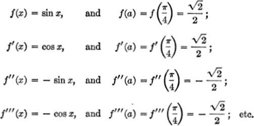
Therefore, substituting in [1]:
EXAMPLE 3. Expand sin (x + h) in terms of powers of h.
Solution. Here f(x + h) = sin (x + h), and f(x) = sin x.
Hence f′(x) = cos x; f″(x) = − sin x; f′″(x) = − cos x; etc.
Substituting in [3]:
![]()
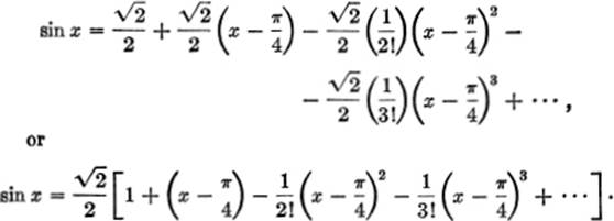
EXAMPLE 4. Expand log (x + h) in terms of powers of h.
Solution. Here f(x + h) = log (x + h); f(x) = log x.
Hence
Substituting in [3]:
![]()
EXERCISE 11—6
1. Expand ex in powers of (x + 3).
2. Expand e−x in powers of (x − 1).
3. Expand sin x in powers of (x − a).
4. Expand cos x in powers of (x − a).
5. Expand log x in powers of (x − a).
6. Expand log x in powers of (x − 3).
7. Expand log (x + h) in powers of x.
8. Expand sin (x + h) in powers of x.
9. Expand cos (x − h) in powers of h.
10. Expand ex+h in powers of h.
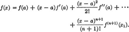
11—19. The Remainder in Taylor’s Series. We may write Taylor’s series with a remainder, as follows:
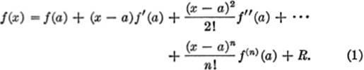
In advanced treatises it is shown that
![]()
where all that we know about x1 is that it lies between a and x. If R → 0 as n → ∞, the Taylor’s series converges and so represents the function in question. The remainder is a measure of the difference between the value of the function f(x) and the sum of the first (n + 1) terms in equation (1).
11—20. Relation of Taylor’s Series to the Theorem of Mean Value. Consider equation (1) of §11—19, with the value of R, as given in equation (2) of the same paragraph, substituted for R in (1). We thus have
If in this equation we take n = 1, we get:
f(x) = f(a)+(x − a) f′(x1). (1)
Now write x = a + h in (1):
f(a + h) = f(a)+ hf′(x1), (2)
where x1 lies between a and (a + h).
Both equations (1) and (2) will be recognized as the law of the mean (§9—3), stated in slightly different form.
11—21. Operations with Power Series. In advanced texts it is shown that power series can be combined under certain conditions. We shall state two of these principles without proof.
I. Two power series may be added for every value of x for which both series converge.
II. A power series may be differentiated term by term for every value of x within the interval of convergence, but not for end-point values of x.
For example:
![]()
differentiating both sides:
![]()