What Is Mathematics? An Elementary Approach to Ideas and Methods, 2nd Edition (1996)

§1. MATTERS OF PRINCIPLE

1. Differentiability

We have linked the concept of derivative of a function y = f(x) with the intuitive idea of tangent to the graph of the function. Since the general concept of function is so wide, it is necessary in the interests of logical completeness to do away with this dependence on geometrical intuition. For we have no guarantee that the intuitive facts familiar from the consideration of simple curves such as circles and ellipses will necessarily subsist for the graphs of more complicated functions. Consider, for example, the function in Figure 282, whose graph has a corner.

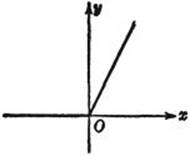
Fig. 282. .

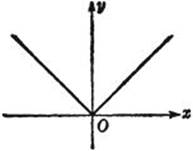
Fig. 283. y = | x |.

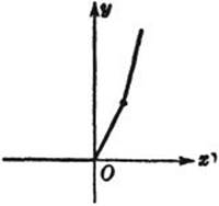
Fig. 284. y = x + | x | + (x – 1) + | x – 1 |.

This function is defined by the equation y = x + | x |, where | x | is the absolute value of x, i.e.

y = x + x = 2x for x ≥ 0,

y = x – x = 0 for x < 0.

Another such example is the function y = | x |; still another is the function y = x + | x | + (x – 1) + | x – 1 |. The graphs of these functions fail to have a definite tangent or direction at certain points; this means that the functions do not possess derivatives for the corresponding values of x.

Exercises: 1) Form the function f(x) whose graph is one-half of a regular hexagon.

2) Where are the corners of the graph of

What are the discontinuities of f′(x)?

For another simple example of non-differentiability, we consider the function

which is obtained from the function sin 1/x (see p. 283) by multiplication by the factor x; we define f(x) to be zero for x = 0. This function, whose graph for positive values of x is shown in Figure 285, is continuous everywhere. The graph oscillates infinitely often in the neighborhood of x = 0, the “waves” becoming very small as we approach x = 0. The slope of these waves is given by

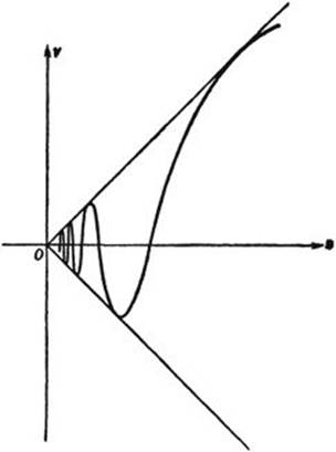
Fig. 285. .

(the reader may verify this as an exercise); as x tends to 0 this slope oscillates between ever-increasing positive and negative bounds. For x = 0 we may try to find the derivative as the limit for h → 0 of the difference quotient

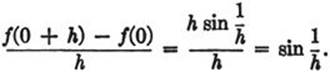
But as h → 0 this difference quotient oscillates between –1 and +1 and does not approach a limit; hence the function cannot be differentiated at x = 0.

These examples indicate a difficulty inherent in the subject. Weierstrass has most strikingly illustrated the situation by constructing a continuous function whose graph does not have a tangent at any point. While differentiability implies continuity, this shows that continuity does not imply differentiability, since Weierstrass’ function is continuous and nowhere differentiable. In practice such difficulties will not arise. Except perhaps for isolated points, curves will be smooth and differentiation will not only be possible but will yield a continuous derivative. Why, then, should we not simply stipulate that “pathological” phenomena are to be absent in problems under consideration? This is exactly what one does in the calculus, where only differentiable functions are considered. In Chapter VIII we carried out the differentiation of a large class of functions and thereby proved their differentiability.

Since the differentiability of a function is not a logical matter of course, it must either be assumed or proved. The concept of tangent or direction of a curve, originally the basis for the concept of derivative, is then derived from the purely analytical definition of derivative: If the function y= f(x) posessses a derivative, i.e. if the difference quotient has a single limit f′(x) as h tends to 0 from either side, then the corresponding curve is said to have a tangent with the slope f′(x). Thus the naive attitude of Fermat, Leibniz, and Newton is reversed in the interests of logical cogency.

Exercises: 1) Show that the continuous function defined by x² sin (1/x) has a derivative at x = 0.

2) Show that the function arc tan (1/x) is discontinuous for x = 0, that x arc tan (1/x) is continuous there but has no derivative, and that x² arc tan (1/x) has a derivative at x = 0.

2. The Integral

The situation is similar with respect to the integral of a continuous function f(x). Instead of considering the “area under the curve” y = f(x) as a quantity which obviously exists and which can be expressed a posteriori as the limit of a sum, we define the integral by this limit, and consider the concept of integral as the primary basis from which the general concept of area is afterward derived. This attitude is forced upon us by a realization of the vagueness of geometrical intuition when applied to analytical concepts as general as that of continuous function. We start by forming a sum

(1)

where x₀ = a, x₁,..., x_n = b is a subdivision of the interval of integration, Δx_j = x_j – x_j–1 is the x-difference or length of the jth subinterval, and v_j is an arbitrary value of x in this subinterval, i.e. x_j–1 ≤ v_j ≤ x_j. (We may take, for example, v_j = x_j or v_j = x_j–1.) Now we form a sequence of such sums in which the number n of subintervals increases and at the same time the maximum length of the subintervals decreases to zero. Then the main fact is: The sum S_n for a given continuous function f(x) tends to a definite limit A, which is independent of the specific way in which the subintervals and points v_j are chosen. By definition, this limit is the integral . Of course, the existence of this limit requires analytical proof if we do not wish to rely on an intuitive geometrical notion of area. This proof is given in every rigorous textbook on the calculus.

Comparing differentiation and integration, we are confronted with the following antithetical situation. Differentiability is definitely a restrictive condition on a continuous function, but the actual carrying out of the differentiation, i.e. the algorithm of the differential calculus, is in practice a straightforward procedure based on a few simple rules. On the other hand, every continuous function without exception possesses an integral between any two given limits. But the explicit calculation of such integrals, even for quite simple functions, is in general a very difficult task. At this point the fundamental theorem of the calculus becomes in many cases the decisive instrument for carrying out the integration. However, for most functions, even for very elementary ones, integration does not yield simple explicit expressions, and the numerical computation of integrals requires advanced methods.

3. Other Applications of the Concept of Integral. Work. Length

Dissociating the analytical notion of integral from its original geometrical interpretation, we meet a number of other, equally important, interpretations and applications. For example, the integral can be interpreted in mechanics as expressing the concept of work. The following simplest case will suffice for our explanation. Suppose a mass moves along the x-axis under the influence of a force directed along the axis. This mass is thought of as concentrated at the point with the coördinate x, and the force is given as a function f(x) of the position, the sign of f(x) indicating whether it points in the positive or negative x-direction. If the force is constant and moves the mass from a to b, then the work done is given by the product, (b – a)f, of the intensity J of the force and the distance traversed by the mass. But if the intensity varies with x, we shall have to define the amount of work done by a limiting process (as we defined velocity). To this end we divide the interval from a to b as before into small subintervals by the points x₀ = a, x₁,..., x_n = b; then we imagine that in each subinterval the force is constant and equal, say, to f(x_y), the actual value at the endpoint, and calculate the work that would correspond to this stepwise varying force:

If we now refine the subdivision as before and let n increase, we see that the sum tends to the integral

Thus the work done by a continuously varying force is defined by an integral.

As an example let us consider a mass m fastened by an elastic spring to the origin x = 0. The force f(x) will, in line with the discussion on page 461, be proportional to x,

f(x) = –k²x,

where k² is a positive constant. Then the work done by this force if the mass moves from the origin to the position x = b will be

and the work we must do against this force, if we want to pull out the spring to this position, is + .

A second application of the general notion of integral is to the concept of arc length of a curve. Let us suppose that the portion of the curve under consideration is represented by a function y = f(x) whose derivative is also a continuous function. To define length we proceedexactly as though we had to measure a curve for practical purposes with a straight yardstick. We inscribe in the arc AB a polygon with n small edges, measure the total length L_n of this polygon, and consider the length L_n as an approximation; letting n increase and the maximum length of the edges of the polygon decrease toward zero, we define

L = lim L_n

as the length of the arc AB. (In Chapter VI the length of a circle was obtained in this way as the limit of the perimeters of inscribed regular n-gons.) It can be shown that for sufficiently smooth curves this limit exists and is independent of the specific way in which the sequence of inscribed polygons is chosen. Curves for which this holds are said to be rectifiable. Any “reasonable” curve that arises in theory or applications will be rectifiable, and we shall not dwell on the investigation of pathological cases. It will suffice to show that the arc AB, for a function y = f(x) with a continuous derivative f′(x), has a length L in this sense, and that L can be expressed by an integral.

To this end, let us denote the x-coördinates of A and B by a and b respectively, then subdivide the x-interval from a to b as before by the points x₀ = a, x₁,..., x_j,..., x_n = b, with the differences Δx_j = x_j – x_j–1, and consider the polygon with the vertices x_i, y_i = f(x_i) above these points of subdivision. A single edge of the polygon will

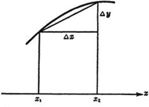
Fig. 286. Arc length.

have the length . Hence we have for the total length of the polygon

If now n tends to infinity, the difference quotients will tend to the derivative and we obtain for the length L the integral expression

(2)  

Without going into further details of this theoretical discussion we make two supplementary remarks. First, if B is considered as a variable point on the curve with the coördinate x, then L = L(x) becomes a function of x, and we have by the fundamental theorem,

a frequently used formula. Second, while formula (2) gives the “general” solution of the problem, it hardly yields an explicit expression for arc length in particular cases. For this we have to substitute the specific function f(x), or rather f′(x), in (2), and then to undertake the actual integration of the expression obtained. Here the difficulty is in general insurmountable if we restrict ourselves to the realm of the elementary functions considered in this book. We shall mention a few cases in which the integration is possible. The function

represents the unit circle; we have , whence , so that the arc length of a circular arc is given by the integral

For the parabola y = x² we have f′(x) = 2x and the arc length from x = 0 to x = b is

For the curve y = log sin x we have f′(x) = cot x and the arc length is expressed by

We shall be content with merely writing down these integral expressions. They could be evaluated with a little more technique than we have at our command, but we shall go no farther in this direction.