What Is Mathematics? An Elementary Approach to Ideas and Methods, 2nd Edition (1996)

§3. INFINITE SERIES AND PRODUCTS

1. Infinite Series of Functions

As we have already stated, expressing a quantity s as an infinite series,

(1)    s = b₁ + b₂ + b₃ +...,

is nothing but a convenient symbolism for the statement that s is the limit, as n increases, of the sequence of finite “partial sums”,

s₁, s₂, s₃,...,

where

(2)   s_n = b₁ + b₂ +... + b_n.

Thus the equation (1) is equivalent to the limiting relation

(3)    lim s_n = s as n→∞,

where s_n is defined by (2). When the limit (3) exists we say that the series (1) converges to the value s, while if the limit (3) does not exist, we say that the series diverges.

Thus, the series

converges to the value π/4, and the series

converges to the value log 2; on the other hand, the series

1 – 1 + 1 – 1 +...

diverges (since the partial sums alternate between 1 and 0), and the series

1 + 1 + 1 + 1 +.

diverges because the partial sums tend to infinity.

We have already encountered series whose terms b_i are functions of x of the form

b_i = c_ixⁱ,

with constant factors c_i. Such series are called power series; they are limits of polynomials representing the partial sums

S_n = c₀ + c₁x + c₂x² +... + c_nxⁿ

(the addition of the constant term c₀ requires an unessential change in the notation (2)). An expansion

f(x) = c₀ + c₁x + c₂x² +...

of a function f(x) in a power series is thus a way of expressing an approximation of f(x) by polynomials, the simplest functions. Summarizing and supplementing previous results, we list the following power series expansions:

(4)

(5)

(6)

(7)

(8)

To this collection we now add the following important expansions:

(9)

(10)

The proof is a simple consequence of the formulas (see p. 440)

(a)   

(b)   

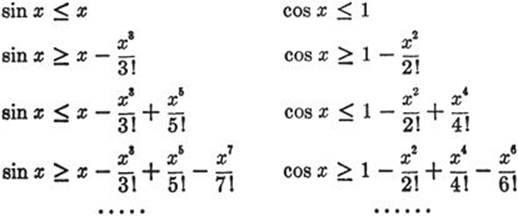
We start with the inequality

cos x ≤ 1.

Integrating from 0 to x, where x is any fixed positive number, we find (see formula (13), p. 414)

sin x ≤ x;

integrating this again,

which is the same thing as

Integrating once more, we obtain

Proceeding indefinitely in this manner, we get the two sets of inequalities

Now xⁿ/n! → 0 as n tends to infinity. To show this we choose a fixed integer m such that , and write c = x^m/m!. For any integer n > m let us set n = m + r; then

and as n → ∞, r also → ∞ and hence ∞ 0. It follows that

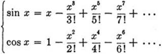
Since the terms, of the series are of alternating sign and decreasing magnitude (at least for | x | ≤ 1), it follows that the error committed by breaking off either series at any term will not exceed in magnitude the value of the first term dropped.

Remarks. These series can be used for the computation of tables. Example: What is sin 1⁰? 1⁰ is π/180 in radian measure; hence

The error committed by breaking off here is not greater than , which is less than 0.000 000 000 02. Hence sin 1⁰ = 0.017 452 406 4, to 10 places of decimals.

Finally, we mention without proof the “binomial series”

(11)

where is the “binomial coefficient”

If a = n is a positive integer, then we have , and for s > n all the coefficients in (11) are zero, so that we simply retain the finite formula of the ordinary binomial theorem. It was one of Newton’s great discoveries, made at the beginning of his career, that the elementary binomial theorem can be extended from positive integral exponents n to arbitrary positive or negative, rational or irrational exponents a. When a is not an integer the right side of (11) yields an infinite series, valid for –1 < x < + 1. For | x | > 1 the series (11) is divergent and thus the equality sign is meaningless.

In particular, we find, by substituting in (11), the expansion

(12)

Like the other mathematicians of the eighteenth century, Newton did not give a real proof for the validity of his formula. A satisfactory analysis of the convergence and range of validity of such infinite series was not given until the nineteenth century.

Exercise: Write the power series for and for .

The expansions (4) – (11) are special cases of the general formula of Brook Taylor (1685–1731), which aims at expanding any one of a large class of functions f(x) in the form of a power series,

(13)  f(x) = c₀ + c₁x + c₂x² + c₃x³ +...,

by finding a law that expresses the coefficients c_i in terms of the function f and its derivatives. It is not possible here to give a precise proof of Taylor’s formula by formulating and establishing the conditions for its validity. But the following plausibility considerations will illuminate the interconnections of the relevant mathematical facts.

Let us tentatively assume that an expansion (13) is possible. Let us further assume that f(x) can be differentiated, that f′(x) can be differentiated, and so on, so that the unending succession of derivatives

f′(x), f″(x),..., f⁽ⁿ⁾(x),...

actually exists. Finally, we take as granted that an infinite power series may be differentiated term by term just like a finite polynomial. Under these assumptions, we can determine the coefficients c_n from a knowledge of the behavior of f(x) in the neighborhood of x = 0. First, by substitutingx = 0 in (13), we find

c₀ = f(0),

since all terms of the series containing x disappear. Now we differentiate (13) and obtain

(13′) f′(x) = c₁ + 2c₂x + 3c₃x² +... + nc_nx^n–1 + ··· .

Again substituting x = 0, but this time in (13′) and not in (13), we find

c₁ = f′(0).

By differentiating (13) we obtain

(13″) f″(x) = 2c₂ + 2·3·c₃x +... + (n–1)·n·c_nx^n–2 +...;

then substituting x = 0 in (13″), we see that

2! c₂ = f″(0).

Similarly, diffrentiating (13″) and then substituting x = 0,

3! c₃ = f′″(0),

and by continuing this procedure, we get the general formula

where f⁽ⁿ⁾(0) is the value of the nth derivative of f(x) at x = 0. The result is the Taylor series

(14)

As an exercise in differentiation the reader may verify that, in examples (4)–(11), the law of formation of the coefficients of a Taylor series is satisfied.

2. Euler’s Formula, cos x + i sin x = e^ix

One of the most fascinating results of Euler’s formalistic manipulations is an intimate connection in the domain of complex numbers between the sine and cosine functions on the one hand, and the exponential function on the other. It should be stated in advance that Euler’s “proof” and our subsequent argument have in no sense á rigorous character; they are typically eighteenth century examples of formal manipulation.

Let us start with De Moivre’s formula proved in Chapter II,

(cos nφ + i sin nφ) = (cos φ + i sin φ)ⁿ.

In this we substitute φ = x/n, obtaining the formula

Now if x is given, then will differ but slightly from cos 0 = 1 for large n; moreover, since

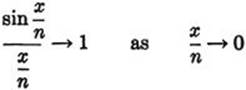
(see p. 307), we see that is asymptotically equal to . We may therefore find it plausible to proceed to the limit formula

(14)

Comparing the right side of this equation with the formula (p. 449)

we have

(15)    cos x + i sin x = e^ix,

which is Euler’s result.

We may obtain the same result in another formalistic way from the expansion of e^z,

by substituting in it z = ix, x being a real number. If we recall that the successive powers of i are i, –1, –i, +1, and so on periodically, then by collecting real and imaginary parts we find

comparing the right hand side with the series for sin x and cos x we again obtain Euler’s formula.

Such reasoning is by no means an actual proof of the relation (15). The objection to our second argument is that the series expansion for e^z was derived under the assumption that z is a real number; therefore the substitution z = ix requires justification. Likewise the validity of the first argument is destroyed by the fact that the formula

e = lim (1 + z/n)ⁿ as n → ∞

was derived for real values of z only.

To remove Euler’s formula from the sphere of mere formalism to that of rigorous mathematical truth required the development of the theory of functions of a complex variable, one of the great mathematical achievements of the nineteenth century. Many other problems stimulated this far-reaching development. We have seen, for example, that the expansions of functions in power series converge for different x-intervals. Why do some expansions converge always, i.e. for all x, while others become meaningless for | x | > 1?

Consider, for example, the geometrical series (4), page 473, which converges for | x | < 1. The left side of this equation is perfectly meaningful when x = 1, taking the value , while the series on the right behaves most strangely, becoming

1 – 1 + 1 – 1 + ···.

This series does not converge, since its partial sums oscillate between 1 and 0. This indicates that functions may give rise to divergent series even when the functions themselves do not show any irregularity. Of course, the function becomes infinite when x → –1. Since it can easily be shown that convergence of a power series for x = a > 0 always implies convergence for –a < x < a, we might find an “explanation” of the queer behavior of the expansion in the discontinuity of for x = − 1. But the function may be expanded into the series

by substituting x² for x in (4). This series will also converge for | x | < 1, while for x = 1 it again leads to the divergent series 1 – 1 + 1 – 1 +..., and for | x | > 1 it diverges explosively, although the function itself is everywhere regular.

It has turned out that a complete explanation of such phenomena is possible only when the functions are studied for complex values of the variable x, as well as for real values. For example, the series for must diverge for x = i because the denominator of the fraction becomes zero. It follows that the series must also diverge for all x such that | x | > | i | = 1, since it can be shown that its convergence for any such x would imply its convergence for x = i. Thus the question of the convergence of series, completely neglected in the early period of the calculus, became one of the main factors in the creation of the theory of functions of a complex variable.

3. The Harmonic Series and the Zeta Function. Euler’s Product for the Sine

Series whose terms are simple combinations of the integers are particularly interesting. As an example we consider the “harmonic series”

(16) 

which differs from that for log 2 by the signs of the even-numbered terms only.

To ask whether this series converges is to ask whether the sequence

s₁, s₂, s₃,...,

where

(17)  

tends to a finite limit. Although the terms of the series (16) approach 0 as we go out farther and farther, it is easy to see that the series does not converge. For by taking enough terms we can exceed any positive number whatever, so that s_n increases without limit and hence the series (16) “diverges to infinity.” To see this we observe that

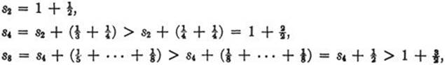
and in general

(18)    

Thus, for example, the partial sums s_2m exceed 100 as soon as m ≥ 200.

Although the harmonic series does not converge, the series

(19) 

may be shown to converge for any value of s greater than 1, and defines for all s > 1 the so-called zeta function,

(20)

as a function of the variable s. There is an important relation between the zeta-function and the prime numbers, which we may derive by using our knowledge of the geometrical series. Let p = 2, 3, 5, 7,... be any prime; then for s ≥ 1,

so that

Let us multiply together these expressions for all the primes p = 2, 3, 5, 7,... without concerning ourselves with the validity of such an operation. On the left we obtain the infinite “product”

while on the other side we obtain the series

by virtue of the fact that every integer greater than 1 can be expressed uniquely as the product of powers of distinct primes. Thus we have represented the zeta-function as a product:

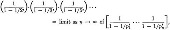
(21)

If there were but a finite number of distinct primes, say p₁, p₂, p₃,..., p_r, then the product on the right side of (21) would be an ordinary finite product and would therefore have a finite value, even for s = 1. But as we have seen, the zeta series for s = 1

diverges to infinity. This argument, which can easily be made into a rigorous proof, shows that there are infinitely many primes. Of course, this is much more involved and sophisticated than the proof given by Euclid (see p. 22). But it has the fascination of a difficult ascent of a mountain peak which could be reached from the other side by a comfortable road.

Infinite products such as (21) are sometimes just as useful as infinite series for representing functions. Another infinite product, whose discovery was one more of Euler’s achievements, concerns the trigonometric function sin x. To understand this formula we start with a remark on polynomials. If f(x) = a₀ + a₁x + . . . + a_nxⁿ is a polynomial of degree n and has n distinct zeros, x₁, ... , x_n then it is known from algebra that f(x) can be decomposed into linear factors:

f(x) = a_n(x – x₁)... (x – x_n).

(see p. 101). By factoring out the product x₁x₂...x_n we can write

where C is a constant which, by setting x = 0, is recognized as C = a₀. Now, if instead of polynomials we consider more complicated functions f(x), the question arises whether a product decomposition by means of the zeros of f(x) is still possible. (In general, this cannot be true, as shown by the example of the exponential function which has no zeros at all, since e^x ≠ 0 for every value of x.) Euler discovered that for the sine function such a decomposition is possible. To write the formula in the simplest way, we consider not sin x, but sin πx. This function has the zeros x = 0, ±1, ±2, ±3,..., since sin πn = 0 for all integers n and for no other numbers. Euler’s formula now states that

(22)

This infinite product converges for all values of x, and is one of the most beautiful formulas in mathematics. For it yields

If we write

we obtain Wallis’ product,

mentioned on page 300.

For proofs of all these facts we must refer the reader to textbooks on the calculus (see also pp. 509–510).