Discrete Fractional Calculus (2015)
1. Basic Difference Calculus
1.10. Stability of Linear Systems
At the outset of this section we will be concerned with the stability of the trivial solution of the vector difference equation
![]()
(1.48)
where A is an n × n constant matrix. By the trivial solution of (1.48) we mean the solution y(t) ≡ 0, ![]() (here by context we know 0 denotes the zero vector). First we define what we mean by the stability of the trivial solution on
(here by context we know 0 denotes the zero vector). First we define what we mean by the stability of the trivial solution on ![]() We will adopt the notation that y(t, z) denotes the unique solution of the IVP
We will adopt the notation that y(t, z) denotes the unique solution of the IVP
![]()
Definition 1.94.
Let ![]() be a norm on
be a norm on ![]() . We say the trivial solution of (1.48) is stable on
. We say the trivial solution of (1.48) is stable on ![]() provided given any ε > 0, there is a δ > 0 such that
provided given any ε > 0, there is a δ > 0 such that ![]() on
on ![]() if
if ![]() If this is not the case we say the trivial solution of (1.48) is unstableon
If this is not the case we say the trivial solution of (1.48) is unstableon ![]() . If the trivial solution is stable on
. If the trivial solution is stable on ![]() and
and ![]() for every solution y of (1.48), then we say the trivial solution of (1.48) is globally asymptotically stable on
for every solution y of (1.48), then we say the trivial solution of (1.48) is globally asymptotically stable on ![]() .
.
We will use the following remark in the proof of the next theorem.
Remark 1.95.
An important result [137, Theorem 2.54] in analysis gives that for any n × n constant matrix M, there is a constant D > 0, depending on M and the norm ![]() on
on ![]() , so that
, so that
![]()
for all ![]() .
.
Theorem 1.96.
If the eigenvalues of A satisfy ![]() , 1 ≤ k ≤ n, then the trivial solution of (1.48) is globally asymptotically stable on
, 1 ≤ k ≤ n, then the trivial solution of (1.48) is globally asymptotically stable on ![]() .
.
Proof.
We will just prove this theorem for the case a = 0. Let ![]() and fix δ so that 0 ≤ r < δ < 1. From the Putzer algorithm (Theorem 1.88), the solution y(t, z) of (1.48) satisfying y(0, z) = z is given by
and fix δ so that 0 ≤ r < δ < 1. From the Putzer algorithm (Theorem 1.88), the solution y(t, z) of (1.48) satisfying y(0, z) = z is given by
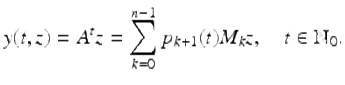
(1.49)
We now show that for each 1 ≤ k ≤ n there is a constant B k > 0 such that
![]()
(1.50)
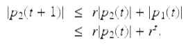
By (1.44),
![]()
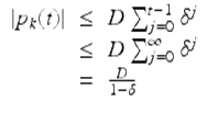
Iterating this inequality and using p 1(0) = 1, we have
![]()
Hence if we let B 1 = 1 and use the fact that r < δ we have that
![]()
Hence (1.50) holds for k = 1. We next show that there is a constant B 2 > 0 such that
![]()
From (1.44) we get
It follows from iteration and p 2(0) = 0 that
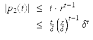
for ![]() . L’Hôpital’s rule implies that
. L’Hôpital’s rule implies that
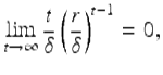
so there is a constant B 2 > 0 so that
![]()
Hence (1.50) holds for k = 2. Similarly, we can show that for ![]()
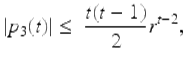
from which it follows that there is a B 3 so that
![]()
Continuing in this manner, we obtain constants B k > 0, 1 ≤ k ≤ n so that
![]()
for k = 1, 2, ⋯ , n. Using Remark 1.95 we have there are constants D k such that
![]()
for all ![]() Using this and (1.49) we have that for
Using this and (1.49) we have that for ![]() ,
,
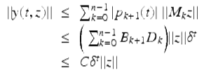
(1.51)
where ![]() . It follows from (1.51) that the trivial solution is stable on
. It follows from (1.51) that the trivial solution is stable on ![]() . Since 0 < δ < 1, it also follows from (1.51) that
. Since 0 < δ < 1, it also follows from (1.51) that ![]() . Hence the trivial solution of (1.48) is globally asymptotically stable on
. Hence the trivial solution of (1.48) is globally asymptotically stable on ![]() . □
. □
Example 1.97.
Consider the vector difference equation
![$$\displaystyle{ u(t+1) = \left [\begin{array}{ll} \;\;1 & - 5\\.25 & - 1 \end{array} \right ]u(t). }$$](fractional.files/image711.png)
(1.52)
The characteristic equation for ![$$A = \left [\begin{array}{ll} \;\;1 & - 5\\.25 & - 1 \end{array} \right ]$$](fractional.files/image712.png) is
is ![]() and hence the eigenvalues of A are
and hence the eigenvalues of A are ![]() and
and ![]() . Since
. Since
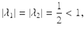
we have by Theorem 1.96 the trivial solution of (1.52) is globally asymptotically stable on ![]() .
.
In the next theorem we give conditions under which the trivial solution of (1.48) is unstable on ![]() .
.
Theorem 1.98.
If there is an eigenvalue, ![]() , of A satisfying
, of A satisfying ![]() , then the trivial solution of (1.48) is unstable on
, then the trivial solution of (1.48) is unstable on ![]() .
.
Proof.
Assume ![]() is an eigenvalue of A so that
is an eigenvalue of A so that ![]() . Let v 0 be a corresponding eigenvector. Then
. Let v 0 be a corresponding eigenvector. Then ![]() is a solution of equation (1.48) on
is a solution of equation (1.48) on ![]() , and
, and
![]()
This implies that the trivial solution of (1.48) is unstable on ![]() . □
. □
Example 1.99.
Consider the vector difference equation
![$$\displaystyle{ y(t+1) = \left [\begin{array}{ll} -.5&\;\;\;3\\ \;\;\;.5 & - 1 \end{array} \right ]y(t). }$$](fractional.files/image722.png)
(1.53)
The characteristic equation for ![$$A = \left [\begin{array}{ll} -.5&\;\;\;3\\ \;\;\;.5 & - 1 \end{array} \right ]$$](fractional.files/image723.png) is
is ![]() and so the eigenvalues are
and so the eigenvalues are ![]()
![]() Since
Since ![]() we have by Theorem 1.98 that the trivial solution of (1.53) is unstable on
we have by Theorem 1.98 that the trivial solution of (1.53) is unstable on ![]()
In the next theorem we give conditions on the matrix A which implies the trivial solution is stable on ![]() .
.
Theorem 1.100.
Let ![]() be the eigenvalues of A. Assume
be the eigenvalues of A. Assume ![]() and whenever
and whenever ![]() , then
, then ![]() is a simple eigenvalue of A. Then the trivial solution of (1.48) is stable on
is a simple eigenvalue of A. Then the trivial solution of (1.48) is stable on ![]() .
.
Proof.
We prove this theorem for the case a = 0. If all the eigenvalues of A satisfy ![]() , then by Theorem 1.96 we have that the trivial solution of (1.48) is stable on
, then by Theorem 1.96 we have that the trivial solution of (1.48) is stable on ![]() . Now assume there is at least one eigenvalue of A with modulus one. Without loss of generality we can order the eigenvalues of A so that
. Now assume there is at least one eigenvalue of A with modulus one. Without loss of generality we can order the eigenvalues of A so that ![]() for
for ![]() , where 2 ≤ k ≤ n and
, where 2 ≤ k ≤ n and ![]() for
for ![]() . From equations (1.44) and (1.45),
. From equations (1.44) and (1.45),
![]()
Next, p 2 satisfies
![]()
so (as in the annihilator method)
![]()
Since ![]() ,
,
![]()
for some constants B 12, B 22. Continuing in this way, we have
![]()
for ![]() . Consequently, there is a constant D > 0 so that
. Consequently, there is a constant D > 0 so that
![]()
for ![]() and
and ![]() .
.
From (1.44), ![]() and hence
and hence
![]()
Choose ![]() . Then
. Then
![]()
By iteration and the initial condition p k (0) = 0,
for ![]() . In a similar manner, we find that there is a constant D ∗ so that
. In a similar manner, we find that there is a constant D ∗ so that
![]()
for ![]() and
and ![]() .
.
From Theorem 1.88, the solution of equation (1.48) satisfying u(0) = u 0, is given by
and it follows that

for ![]() and some C > 0. □
and some C > 0. □
Example 1.101.
Consider the system
![$$\displaystyle{ u(t+1) = \left [\begin{array}{ll} \;\;\;\cos \theta &\sin \theta \\ -\sin \theta &\cos \theta \end{array} \right ]u(t),\quad t \in \mathbb{N}_{ a}, }$$](fractional.files/image752.png)
(1.54)
where ![]() is a real number. For each
is a real number. For each ![]() the eigenvalues of the coefficient matrix in (1.54) are
the eigenvalues of the coefficient matrix in (1.54) are ![]() Since
Since ![]() and both eigenvalues are simple, we have by Theorem 1.100 that the trivial solution of (1.54) is stable on
and both eigenvalues are simple, we have by Theorem 1.100 that the trivial solution of (1.54) is stable on ![]() . From linear algebra the coefficient matrix in (1.54) is called a rotation matrix. When a vector u is multiplied by this coefficient matrix, the resulting vector has the same length as u, but its direction is
. From linear algebra the coefficient matrix in (1.54) is called a rotation matrix. When a vector u is multiplied by this coefficient matrix, the resulting vector has the same length as u, but its direction is ![]() radians clockwise from u. Consequently, every solution u of the system has all of its values on a circle centered at the origin of radius | u(a) | . This also tells us that the trivial solution of (1.54) is stable on
radians clockwise from u. Consequently, every solution u of the system has all of its values on a circle centered at the origin of radius | u(a) | . This also tells us that the trivial solution of (1.54) is stable on ![]() but not globally asymptotically stable on
but not globally asymptotically stable on ![]()