Discrete Fractional Calculus (2015)
1. Basic Difference Calculus
1.12. Exercises
1.1. Show that if ![]() satisfies
satisfies ![]() for
for ![]() , then f(t) = C for
, then f(t) = C for ![]() , where C is a constant.
, where C is a constant.
1.2. Prove the product rules
(i)
![]()
(ii)
![]()
Why does (i) imply (ii)?
1.3. Show that ![]() and that for any positive integer that
and that for any positive integer that ![]()
1.4. Show that for x a real variable that ![]()
1.5. Show that ![]() Hint first show that
Hint first show that

1.6. By Exercise 1.5, ![]() . Find
. Find ![]() and
and ![]()
1.7. Use the definition of the (generalized) falling function (Definition 1.7) to show that for ![]() ,
,
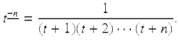
Then use this expression directly (do not use the gamma function) to prove
![]()
![]()
1.8. Show that ![]() for
for ![]() , and that
, and that ![]() , ν − k ≠ − 1, −2, −3, ⋯ , k = 1, 2, 3, ⋯ .
, ν − k ≠ − 1, −2, −3, ⋯ , k = 1, 2, 3, ⋯ .
1.9. Show that
![]()
whenever both sides of this equation are well defined.
1.10. For integers m and n satisfying m > n ≥ 0, evaluate the binomial coefficient ![]()
1.11. Evaluate each of the following binomial coefficients:
(i)
![]() for
for ![]()
(ii)
![]()
(iii)
![]()
(iv)
![]()
1.12. Prove each of the following:
(i)
![]()
(ii)
![]()
(iii)
![]()
(iv)
![]()
(v)
![]()
where in (iv) ν > 0 and ![]()
1.13. Prove Theorem 1.10.
1.14. For each of the following, find e p (t, a) given that
(i)
![]()
(ii)
![]()
(iii)
![]()
(iv)
![]()
1.15. Let P(t) be the population of a bacteria in a culture after t hours. Assuming that P satisfies the IVP
![]()
use Theorem 1.14 to find a formula for P(t).
1.16 (Compound Interest). A bank pays interest with an annual interest rate of 8% and interest is compounded 4 times a year. If $100 is invested, how much money do you have after 20 years?
1.17 (Radioactive Decay). Let R(t) be the amount of the radioactive isotope Pb-209 present at time t. Assume initially that R 0 is the amount of Pb-209 present and that the change in the amount of Pb-209 each hour is proportional to the amount present at the beginning of that hour and the half life of Pb-209 is 3.3 hours. Find a formula for R(t). How long does it take for 70% of the Pb-209 to decay?
1.18. Show that if ![]() , then
, then

1.19. Complete the proof of Theorem 1.16 by showing that the addition ⊕ on ![]() is associative and commutative.
is associative and commutative.
1.20. Show that the set of positively regressive functions ![]() with the addition ⊕ is a subgroup of the set of regressive functions
with the addition ⊕ is a subgroup of the set of regressive functions ![]()
1.21. Prove Theorem 1.21 if a is replaced by s, where ![]()
1.22. Prove parts (iv) and (v) of Theorem 1.25.
1.23. Prove part (ii) of Theorem 1.27.
1.24. Prove that if ![]() and
and ![]() , then
, then
![]()
where the right-hand side has n terms.
1.25. Prove that if ![]() and
and ![]() , then the following hold:
, then the following hold:
(i)
α ⊙ (β ⊙ p) = (α β) ⊙ p;
(ii)
α ⊙ (p ⊕ q) = (α ⊙ p) ⊕ (α ⊙ q).
1.26. Prove Theorem 1.28 directly (do not use Theorem 1.27) from the definitions of ![]() and
and ![]() .
.
1.27. Derive Euler’s formula (1.11)
![]()
Also derive the hyperbolic analogue of Euler’s formula
![]()
1.28. Verify each of the following formulas for p ≠ ± i:
(i)
![]()
(ii)
![]()
(iii)
![]()
(iv)
![]()
1.29. Prove Theorem 1.40.
1.30. Prove Theorem 1.42.
1.31. Using a delta integral (see Example 1.57) find
(i)
the sum of the first n positive integers;
(ii)
the sum of the cubes of the first n positive integers.
1.32. Show by direct substitution that y(t) = (t − a)e r (t, a), r ≠ − 1, is a solution of the second order linear equation ![]()
1.33. Solve each of the following difference equations:
(i)
![]()
(ii)
![]()
(iii)
![]()
(iv)
![]()
(v)
![]()
(vi)
![]()
1.34. Solve each of the following difference equations:
(i)
![]()
(ii)
![]()
(iii)
![]()
1.35. Solve each of the following linear difference equations:
(i)
![]()
(ii)
![]()
1.36. Show that a second order linear homogeneous equation of the form ![]() with p(t) ≠ 1 + q(t) is equivalent to an equation of the form y(t + 2) + c(t)y(t + 1) + d(t)y(t) = 0 with d(t) ≠ 0.
with p(t) ≠ 1 + q(t) is equivalent to an equation of the form y(t + 2) + c(t)y(t + 1) + d(t)y(t) = 0 with d(t) ≠ 0.
1.37 (Real Roots). Find the value of the determinant of the t by t matrix with all 4’s on the diagonal, 1’s on the superdiagonal, 3’s on the subdiagonal, and 0’s elsewhere.
1.38 (Complex Roots). Find the value of the determinant of the t by t matrix with all − 2’s on the diagonal, 4’s on the superdiagonal, 1’s on the subdiagonal, and 0’s elsewhere.
1.39 (Complex Roots). Find the value of the determinant of the t by t matrix with all 2’s on the diagonal, 4’s on the superdiagonal, 1’s on the subdiagonal, and 0’s elsewhere.
1.40. What would you guess are general solutions of each of the following:
(i)
![]()
(ii)
![]()
(iii)
![]()
1.41. Show that if F(t) is the t-th term in the Fibonacci sequence (see Example 1.32), then
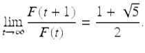
The ratio ![]() is known as the “golden section” and was considered by the ancient Greeks to be the most aesthetically pleasing ratio of the length of a rectangle to its width.
is known as the “golden section” and was considered by the ancient Greeks to be the most aesthetically pleasing ratio of the length of a rectangle to its width.
1.42. In how many ways can you tile a 1 × n, hallway, n ≥ 2, if you have green 1 × 1 tiles and red and yellow 1 × 2 tiles?
1.43. Solve the following difference equations:
(i)
![]()
(ii)
![]()
(iii)
![]()
1.44. Solve the following difference equations:
(i)
![]()
(ii)
![]()
(iii)
![]()
1.45. Solve the following difference equations:
(i)
![]()
(ii)
![]()
(iii)
![]()
(iv)
![]()
1.46. Use the method of annihilators to solve the following difference equations:
(i)
![]()
(ii)
![]()
(iii)
![]()
1.47. Use the method of annihilators to solve the following difference equations:
(i)
![]()
(ii)
![]()
(iii)
![]()
1.48. Use integration by parts to evaluate each of the following:
(i)
![]()
(ii)
![]()
(iii)
![]()
1.49. Evaluate ![]() for
for ![]()
1.50. Use integration by parts to evaluate each of the following:
(i)
![]()
(ii)
![]()
(iii)
![]()
1.51. Show directly (do not use Theorem 1.62) that if ![]() is a polynomial of degree n, then
is a polynomial of degree n, then ![]() here h k (t, a),
here h k (t, a), ![]() are the Taylor monomials.
are the Taylor monomials.
1.52. Solve the IVP in Example 1.66 by twice integrating both sides of ![]() from 0 to t.
from 0 to t.
1.53 (Tower of Hanoi Problem). Assume you have three vertical pegs with n rings of different sizes on the first peg with larger rings below smaller ones. Find the minimum number of moves, y(n), that it takes in moving the nrings on the first peg to the third peg. A move consists of transferring a single ring from one peg to another peg with the restriction that a larger ring cannot be placed on a smaller ring. (Hint: Find a first order linear equation that y(n) satisfies and use Theorem 1.68 to find y(n). )
1.54. Suppose that at the beginning of each year we deposit $2, 000 dollars in an IRA account that pays an annual interest rate of 4%. Find an IVP that the amount of money, y(t), that we have in the account after t years satisfies and use Theorem 1.68 to find y(t). How much money do we have in the account after 25 years?
1.55. Suppose at the beginning of each year that we deposit $3, 000 dollars in an IRA account that pays an annual interest rate of 5%. How much money, y(t), will we have in our IRA account at the end of the t-th year?
1.56. Prove that the IVP in Theorem 1.68 has a unique solution on ![]() .
.
1.57 (Newton’s Law of Cooling). A small object of temperature 70 degrees F is placed at time t = 0 in a large body of water with constant temperature 40 degrees F. After 10 minutes the temperature of the object is 60 degrees F. Experiments indicate that during each minute the change in the temperature of the object is proportional to the difference of the temperature of the object and the water at the beginning of that minute. What is the temperature of the object after 5 minutes? When will the temperature of the object be 50 degrees F?
1.58. Solve each of the following first order linear difference equations
(i)
![]()
(ii)
![]()
(iii)
![]()
(iv)
![]()
where in (iii) we assume ![]()
1.59. Solve each of the following first order linear difference equations
(i)
![]()
(ii)
![]()
1.60. Show that the operators ![]() and
and ![]() , where I is the identity operator, as operators on the set of functions mapping
, where I is the identity operator, as operators on the set of functions mapping ![]() to
to ![]() do not commute.
do not commute.
1.61. Show that the operators ![]() and
and ![]() commute, where I is the identity operator and α and β are constants, as operators on the set of functions mapping
commute, where I is the identity operator and α and β are constants, as operators on the set of functions mapping ![]() to
to ![]() .
.
1.62. Use the method of factoring to solve each of the following difference equations:
(i)
![]()
(ii)
![]()
(iii)
![]()
(iv)
![]()
1.63. Use the method of factoring to solve each of the following difference equations:
(i)
![]()
(ii)
![]()
1.64. Solve the following Euler–Cauchy difference equations:
(i)
![]()
(ii)
![]()
1.65. Solve the following Euler–Cauchy difference equations:
(i)
![]()
(ii)
![]()
(iii)
![]()
1.66. Solve the following Euler–Cauchy difference equations:
(i)
![]()
(ii)
![]()
(iii)
![]()
1.67. Solve the following Euler–Cauchy difference equations:
(i)
![]()
(ii)
![]()
1.68. Prove Theorem 1.86.
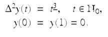
1.69. Use the variation of constants formula as in Example 1.66 to solve the IVP
1.70. Use the variation of constants formula as in Example 1.66 to solve the IVP
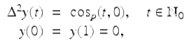
where p ≠ 0, ±i is a constant.
1.71. Assume A(t) is a regressive matrix function on ![]() . Show that
. Show that ![]() is a fundamental matrix of
is a fundamental matrix of ![]() if and only if its columns are n linearly independent solutions of the vector equation
if and only if its columns are n linearly independent solutions of the vector equation ![]() on
on ![]() .
.
1.72. Show that
![$$\displaystyle\begin{array}{rcl} \Phi (t)&:=& \left [\begin{array}{ll} (-2)^{t} &(-1)^{t} \\ (-2)^{t+1} & (-1)^{t+1} \end{array} \right ] {}\\ & =& (-1)^{t}\left [\begin{array}{ll} \;\;\;2^{t} &\;\;1 \\ - 2^{t+1} & - 1 \end{array} \right ]{}\\ \end{array}$$](fractional.files/image973.png)
is a fundamental matrix of the system
![$$\displaystyle{u(t+1) = \left [\begin{array}{ll} \;\;0 &\;\;1\\ - 2 & - 3 \end{array} \right ]u(t).}$$](fractional.files/image974.png)
1.73. Prove Theorem 1.82.
1.74. Prove that if A(t) is a regressive matrix function on ![]() , then
, then
![]()
for ![]() .
.
1.75. Show that if Y (t) is invertible for ![]() , then
, then
![]()
for ![]()
1.76. For each of the following show directly that the given matrix satisfies its own characteristic equation.
(i)
![$$A = \left [\begin{array}{*{10}c} \;\;2 & \;\;1 &3\\ -1 & \;\;2 &0 \\ \;\;1 &-2&3\end{array} \right ];$$](fractional.files/image978.png)
(ii)
![$$A = \left [\begin{array}{*{10}c} a&b\\ c &d\end{array} \right ].$$](fractional.files/image979.png)
1.77. Find 2 by 2 matrices A and B such that A t B t ≠ (AB) t for some t ≥ 1. Show that if two n by n matrices C and D commute, then (CD) t = C t D t for t = 0, 1, 2, ⋯ .
1.78. Prove part (viii) of Theorem 1.84, that is
![]()
where A ∗ denotes the conjugate transpose of the matrix A.
1.79. Prove part (ix) of Theorem 1.84, that is B(t)e A (t, t 0) = e A (t, t 0)B(t), if A(t) and B(τ) commute for all ![]()
1.80. Solve each of the following systems:
(i)
![$$u(t+1) = \left [\begin{array}{*{10}c} 1&-1\\ 1 & \;\;1\end{array} \right ]u(t);$$](fractional.files/image982.png)
(ii)
![$$u(t+1) = \left [\begin{array}{*{10}c} 1&-4\\ 2 &\;-3\end{array} \right ]u(t);$$](fractional.files/image983.png)
(iii)
![$$u(t+1) = \left [\begin{array}{*{10}c} 8&-4&0\\ 9 &-4 &0 \\ 2&-1&3\end{array} \right ]u(t);$$](fractional.files/image984.png)
(iv)
![$$u(t+1) = \left [\begin{array}{*{10}c} 1&0&0\\ 1 &0 &1 \\ 0&1&0\end{array} \right ]u(t).$$](fractional.files/image985.png)
1.81. Solve each of the following IVPs:
(i)
![$$u(t+1) = \left [\begin{array}{*{10}c} \;\;1 &1\\ -1 &3\end{array} \right ]u(t),\quad u(0) = \left [\begin{array}{*{10}c} \;\;2\\ -1\end{array} \right ];$$](fractional.files/image986.png)
(ii)
![$$u(t+1) = \left [\begin{array}{*{10}c} 2&0\\ 0 &1\end{array} \right ]u(t)+\left [\begin{array}{*{10}c} 2^{t} \\ 3^{t}\end{array} \right ],\quad u(0) = \left [\begin{array}{*{10}c} 1\\ 2\end{array} \right ];$$](fractional.files/image987.png)
(iii)
![$$u(t+1) = \left [\begin{array}{*{10}c} \;\;\;2 &1\\ -1 &4\end{array} \right ]u(t)+\left [\begin{array}{*{10}c} \;3^{-t} \\ 0\end{array} \right ],\quad u(0) = \left [\begin{array}{*{10}c} \;\;1\\ -1\end{array} \right ].$$](fractional.files/image988.png)
1.82. Solve each of the following IVPs:
(i)
![$$u(t+1) = \left [\begin{array}{*{10}c} \;\;4 &1\\ -1 &2\end{array} \right ]u(t)+\left [\begin{array}{*{10}c} 1\\ 2\end{array} \right ],\ \ u(0)\ =\ \left [\begin{array}{*{10}c} 1\\ -1\end{array} \right ];$$](fractional.files/image989.png)
(ii)
![$$u(t+1) = \left [\begin{array}{*{10}c} 2& \;\;2\\ 2 &-1\end{array} \right ]u(t)+\left [\begin{array}{*{10}c} 1\\ 0\end{array} \right ],\ \ u(0)\ =\ \left [\begin{array}{*{10}c} 1\\ 1\end{array} \right ];$$](fractional.files/image990.png)
(iii)
![$$u(t+1) = \left [\begin{array}{*{10}c} -1&4\\ -3 &6\end{array} \right ]u(t)+\left [\begin{array}{*{10}c} 0\\ 3^{t}\end{array} \right ],\ \ u(0)\ =\ \left [\begin{array}{*{10}c} 1\\ 1\end{array} \right ].$$](fractional.files/image991.png)
1.83. Use Putzer’s algorithm (see Example 1.89) to find e A (t, 0) for each of the following:
(i)
![$$A = \left [\begin{array}{*{10}c} \;3 &1\\ -1 &\;1\end{array} \right ];$$](fractional.files/image992.png)
(ii)
![$$A = \left [\begin{array}{*{10}c} 0&-1\\ 1 & \;2\end{array} \right ];$$](fractional.files/image993.png)
(iii)
![$$A = \left [\begin{array}{*{10}c} \;2 &1\\ -1 &\;2\end{array} \right ].$$](fractional.files/image994.png)
1.84. Let
![$$\displaystyle{A = \left [\begin{array}{*{10}c} \;\;0 & \;\;1\\ -c &\;-d \end{array} \right ].}$$](fractional.files/image995.png)
Show that if the matrix A has a multiple characteristic root with modulus one, then the vector equation y(t + 1) = Ay(t), ![]() , has an unbounded solution and hence the trivial solution of y(t + 1) = Ay(t) is unstable on
, has an unbounded solution and hence the trivial solution of y(t + 1) = Ay(t) is unstable on ![]() Relate this example to Theorem 1.100.
Relate this example to Theorem 1.100.
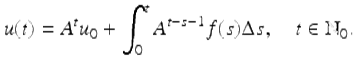
1.85. Prove the following result. Assume A is an n × n constant matrix and ![]() . Then the solution of the IVP
. Then the solution of the IVP
![]()
(1.61)
where u 0 is a given n × 1 constant vector has a unique solution given by
1.86. Without solving y(t + 1) = Ay(t), ![]() determine the stability of the trivial solution of y(t + 1) = Ay(t) on
determine the stability of the trivial solution of y(t + 1) = Ay(t) on ![]() for each of the following cases:
for each of the following cases:
(i)
![$$A = \left [\begin{array}{*{10}c} \;\;\;0 &1\\ -\frac{1} {2} & \;1\end{array} \right ];$$](fractional.files/image1000.png)
(ii)
![$$A = \left [\begin{array}{*{10}c} 0 & 1\\ \frac{1} {6} & \;\frac{1} {6}\end{array} \right ];$$](fractional.files/image1001.png)
(iii)
![$$A = \left [\begin{array}{*{10}c} \frac{1} {2} & \;\;\;0 & 0 \\ 0 & \;\;\;\frac{1} {2} & \frac{2} {3} \\ 0 &-\frac{2} {3} & \frac{1} {2}\end{array} \right ].$$](fractional.files/image1002.png)
1.87. Find the Floquet multiplier of each of the following difference equations:
(i)
![]()
(ii)
![]()
1.88. Find the Floquet multipliers of the Floquet system
![$$\displaystyle{u(t+1) = \left [\begin{array}{ll} \quad \;0 &1 + \frac{3+(-1)^{t}} {2} \\ \frac{3-(-1)^{t}} {2} & \quad \quad 0 \end{array} \right ]u(t).}$$](fractional.files/image1005.png)
1.89. Show that if ![]() are distinct Floquet multipliers, then there are k linearly independent solutions, y i (t), 1 ≤ i ≤ k, of the Floquet system (1.55) on
are distinct Floquet multipliers, then there are k linearly independent solutions, y i (t), 1 ≤ i ≤ k, of the Floquet system (1.55) on ![]() satisfying
satisfying
![]()
1.90. Find the Floquet multipliers of the Floquet system
![$$\displaystyle{u(t+1) = \left [\begin{array}{ll} \quad \;1 &\sin \left ( \frac{\pi }{2}t\right ) \\ \cos \left ( \frac{\pi }{2}t\right )&\quad \quad 1 \end{array} \right ]u(t),\quad t \in \mathbb{Z}_{0}.}$$](fractional.files/image1009.png)
1.91. Find the Floquet multipliers of the Floquet system
![$$\displaystyle{u(t+1) = \left [\begin{array}{ll} \quad \;1 &\sin \left (\frac{2\pi } {3}t\right ) \\ \cos \left (\frac{2\pi } {3}t\right )&\quad \quad 1 \end{array} \right ]u(t),\quad t \in \mathbb{Z}_{0}.}$$](fractional.files/image1010.png)
1.92. Prove Theorem 1.113.
Bibliography
63.
Bohner, M., Peterson, A.: Advances in Dynamic Equations on Time Scales. Birkhäuser, Boston, MA (2003)CrossRefMATH
87.
Gautschi, W.: Zur numerik rekurrenten relationen. Computing 9, 107–126 (1972)CrossRefMathSciNetMATH
134.
Kelley, W.G., Peterson, A.C.: Difference Equations: An Introduction with Applications, First Edition. Academic Press, New York (1991)MATH
135.
Kelley, W.G., Peterson, A.C.: Difference Equations: An Introduction with Applications, Second Edition. Academic Press, New York (2001)
137.
Kelley, W.G., Peterson, A.C.: The Theory of Differential Equations: Classical and Qualitative, Second Edition. Universitext, Springer, New York (2010)CrossRef
152.
Oldham, K., Spanier, J.: The Fractional Calculus: Theory and Applications of Differentiation and Integration to Arbitrary Order. Dover Publications, Mineola, New York (2002)