Discrete Fractional Calculus (2015)
2. Discrete Delta Fractional Calculus and Laplace Transforms
2.6. The Convolution Product
The following definition of the convolution product agrees with the convolution product defined for general time scales in [62], but it differs from the convolution product defined by Atici and Eloe in [32] (in the upper limit). We demonstrate several advantages of using Definition 2.59 in the following results.
Definition 2.59.
Let ![]() be given. Define the convolution product of f and g to be
be given. Define the convolution product of f and g to be

(2.42)
(note that ![]() by our convention on sums).
by our convention on sums).
Example 2.60.
For p ≠ 0, −1, find the convolution product e p (t, a) ∗ 1, and use your answer to find ![]() By the definition of the convolution product
By the definition of the convolution product
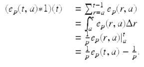
It follows that
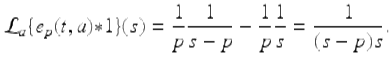
Note from Example 2.60 we get that

which is a special case of the following theorem which gives a formula for the Laplace transform of the convolution product of two functions. Later we will show that this formula is useful in solving fractional initial value problems. In this theorem we use the notation ![]() which was introduced earlier.
which was introduced earlier.
Theorem 2.61 (Convolution Theorem).
Let ![]() be of exponential order r 0 > 0. Then
be of exponential order r 0 > 0. Then
![]()
(2.43)
Proof.
We have
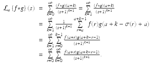
Making the change of variables ![]() gives us that
gives us that
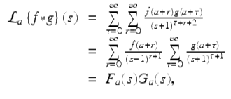
for | s + 1 | > r 0. □
Example 2.62.
Solve the (Volterra) summation equation
![$$\displaystyle{ y(t) = 3 + 12\sum _{r=0}^{t-1}\;\left [2^{t-r-1} - 1\right ]\;y(r),\quad t \in \mathbb{N}_{ 0} }$$](fractional.files/image1366.png)
(2.44)
using Laplace transforms. We can write equation (2.44) in the equivalent form
![$$\displaystyle\begin{array}{rcl} y(t)& =& 3 + 12\;\sum _{r=0}^{t-1}[e_{ 1}(t - r - 1,0) - 1]y(r) \\ & =& 3 + 12\;[(e_{1}(t,0) - 1) {\ast} y(t)],\quad t \in \mathbb{N}_{0}.{}\end{array}$$](fractional.files/image1367.png)
(2.45)
Taking the Laplace transform (based at 0) of both sides of (2.45), we obtain
![$$\displaystyle\begin{array}{rcl} Y _{0}(s)& =& \frac{3} {s} + 12\;\left [ \frac{1} {s - 1} -\frac{1} {s}\right ]\;Y _{0}(s) {}\\ & =& \frac{3} {s} + \frac{12} {s(s - 1)}Y _{0}(s). {}\\ \end{array}$$](fractional.files/image1368.png)
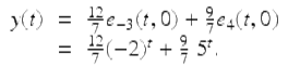
Solving for Y 0(s), we get
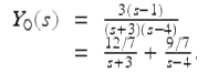
Taking the inverse Laplace transform of both sides, we get