Discrete Fractional Calculus (2015)
2. Discrete Delta Fractional Calculus and Laplace Transforms
2.10. The Laplace Transform Method
The tools developed in the previous sections of this chapter enable us to solve a general fractional initial value problem using the Laplace transform. The initial value problem (2.53) below is identical to that studied and solved using the composition rules in Holm [123, 125]. In Theorem 2.76 below, we present only that part of the proof involving the Laplace transform method.
Theorem 2.73.
Assume ![]() is of exponential order r ≥ 1 and ν > 0 with N − 1 < ν ≤ N. Then the unique solution of the IVP
is of exponential order r ≥ 1 and ν > 0 with N − 1 < ν ≤ N. Then the unique solution of the IVP
is given by
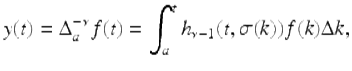
for ![]()
Proof.
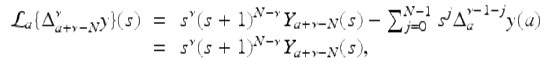
Since
![]()
we have that
![]()
for | s + 1 | > r. Assume for the moment that the Laplace transform (based at ![]() ) of the solution of the given IVP converges for | s + 1 | > r. It follows from (2.52) that
) of the solution of the given IVP converges for | s + 1 | > r. It follows from (2.52) that
where we have used the initial conditions. It follows that
It then follows from the uniqueness theorem for Laplace transforms, Theorem 2.7, that
![]()
From this we now know that y is of exponential order r and hence the above arguments hold and the proof is complete. □
Using Theorem 2.73 and Theorem 2.43 it is easy to prove the following result.
Theorem 2.74.
Assume ![]() is of exponential order r ≥ 1 and ν > 0 with N − 1 < ν ≤ N. Then a general solution of the nonhomogeneous equation
is of exponential order r ≥ 1 and ν > 0 with N − 1 < ν ≤ N. Then a general solution of the nonhomogeneous equation
![]()
is given by
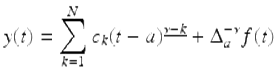
for ![]()
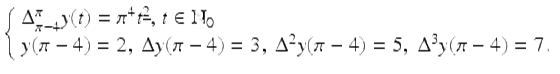
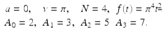
Example 2.75.
Solve the IVP
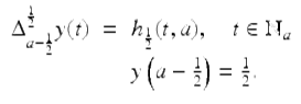
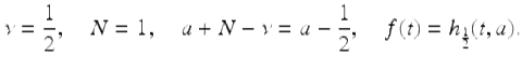
Note this IVP is of the form of the IVP in Theorem 2.74, where
From Theorem 2.74 a general solution of the fractional equation 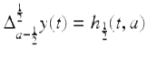 is given by
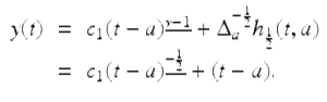
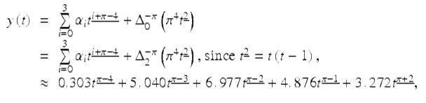
Applying the initial condition we get ![]() Hence the solution of the given IVP in this example is given by
Hence the solution of the given IVP in this example is given by
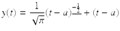
for ![]()
The following theorem appears in Ahrendt et al. [3].
Theorem 2.76.
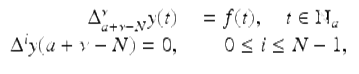
Suppose that ![]() is of exponential order r ≥ 1, and let ν > 0 be given with N − 1 < ν ≤ N. The unique solution to the fractional initial value problem
is of exponential order r ≥ 1, and let ν > 0 be given with N − 1 < ν ≤ N. The unique solution to the fractional initial value problem
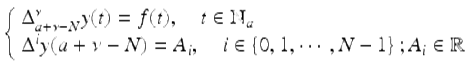
(2.53)
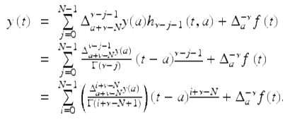
is given by
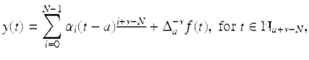
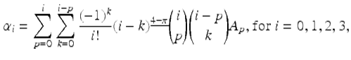
where
for ![]()
Proof.
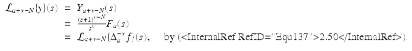
Since f is of exponential order r, we know that ![]() exists for | s + 1 | > r. So, applying the Laplace transform to both sides of the difference equation in (2.53), we have for | s + 1 | > r
exists for | s + 1 | > r. So, applying the Laplace transform to both sides of the difference equation in (2.53), we have for | s + 1 | > r
![]()
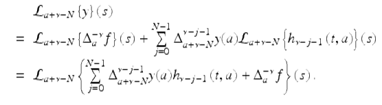
Using (2.52), we get
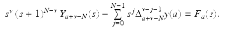
This implies that
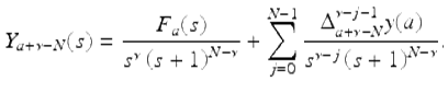
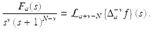
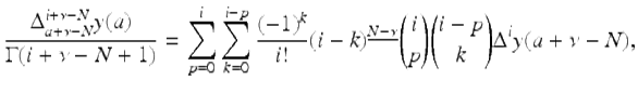
From (2.50), we have immediately that
Considering next the terms in the summation, we have for each fixed j ∈ { 0, ⋯ , N − 1},
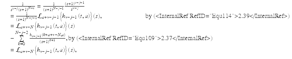
since
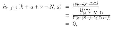
for ![]() It follows that for | s + 1 | > r,
It follows that for | s + 1 | > r,
Since the Laplace transform is injective, we conclude that for ![]()
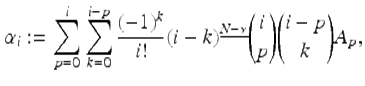
Moreover, Holm [125] showed that
for ![]() concluding the proof. □
concluding the proof. □
Theorem 2.76 shows how we can solve the general IVP (2.53) using the discrete Laplace transform method. We offer a brief example.
Example 2.77.
Consider the IVP given by
(2.54)
Note that (2.54) is a specific case of (2.53) from Theorem 2.76, with
After applying the discrete Laplace transform method as described in Theorem 2.76, we have
where in this last step, we calculated
for the first four terms and applied the power rule (Theorem 2.71) on the last term.