Discrete Fractional Calculus (2015)
1. Basic Difference Calculus
1.4. Second Order Linear Equations with Constant Coefficients
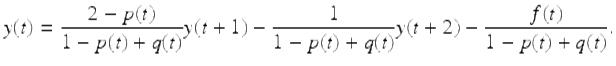
The nonhomogeneous second order linear difference equation is given by
![]()
(1.12)
where we assume that p(t) ≠ q(t) + 1, for ![]() In this section we will see that we can easily solve the corresponding second order linear homogeneous equation with constant coefficients
In this section we will see that we can easily solve the corresponding second order linear homogeneous equation with constant coefficients
![]()
(1.13)
where we assume the constants ![]() satisfy p ≠ 1 + q.
satisfy p ≠ 1 + q.
First we prove an existence-uniqueness theorem for solutions of initial value problems (IVPs) for (1.12).
Theorem 1.29.
Assume that ![]() , p(t) ≠ 1 + q(t),
, p(t) ≠ 1 + q(t), ![]() ,
, ![]() and
and ![]() Then the IVP
Then the IVP
![]()
(1.14)
has a unique solution y(t) on ![]()
Proof.
Expanding equation (1.12) out we have first solving for y(t + 2) and then solving for y(t) that
![]()
(1.15)
and, since p(t) ≠ 1 + q(t), ![]() ,
,
(1.16)
If we let t = t 0 in (1.15), then equation (1.12) holds at t = t 0 iff
![]()
Hence, the solution of the IVP (1.14) is uniquely determined at t 0 + 2. But using the equation (1.15) evaluated at t = t 0 + 1, we have that the unique values of the solution at y(t 0 + 1) and y(t 0 + 2) uniquely determines the value of the solution at t 0 + 3. By induction we get that the solution of the IVP (1.14) is uniquely determined on ![]() . On the other hand, if t 0 > a, then using equation (1.16) with t = t 0 − 1, we have that
. On the other hand, if t 0 > a, then using equation (1.16) with t = t 0 − 1, we have that
![$$\displaystyle{y(t_{0} - 1) = \frac{1} {1 - p(t_{0} - 1) + q(t_{0} - 1)}\bigg[[2 - p(t_{0} - 1)]A - B - f(t_{0} - 1)\bigg].}$$](fractional.files/image208.png)
Hence the solution of the IVP (1.14) is uniquely determined at t 0 − 1. Proceeding in this manner we have by mathematical induction that the solution of the IVP (1.14) is uniquely determined on ![]() Hence the result follows. □
Hence the result follows. □
Remark 1.30.
It follows from Theorem 1.29, that if p(t) ≠ 1 + q(t), ![]() , then the general solution of the linear homogeneous equation
, then the general solution of the linear homogeneous equation
![]()
is given by
![]()
where y 1(t), y 2(t) are any two linearly independent solutions of (1.13) on ![]()
We now show we can solve the second order linear homogeneous equation (1.13) with constant coefficients.
Theorem 1.31 (Distinct Roots).
Assume p ≠ 1 + q and ![]() (possibly complex) are solutions (called the characteristic values of (1.13) ) of the characteristic equation
(possibly complex) are solutions (called the characteristic values of (1.13) ) of the characteristic equation
![]()
Then
![]()
is a general solution of (1.13) .
Proof.
Assume ![]()
![]() are characteristic values of (1.13). Then the characteristic equation of (1.13) is given by
are characteristic values of (1.13). Then the characteristic equation of (1.13) is given by
![]()
It follows that ![]() and
and ![]() . Hence
. Hence ![]()
![]() , since p ≠ q + 1. Hence, we have that
, since p ≠ q + 1. Hence, we have that ![]() and so
and so ![]() , i = 1, 2, are well defined. Since
, i = 1, 2, are well defined. Since
![]()
we have that ![]() , i = 1, 2, are solutions of (1.13). Since these two solutions are linearly independent on
, i = 1, 2, are solutions of (1.13). Since these two solutions are linearly independent on ![]() , we have that
, we have that
![]()
is a general solution of (1.13) on ![]() . □
. □
Example 1.32 (Fibonacci Numbers).
The Fibonacci numbers F(t), t = 1, 2, 3, ⋯ are defined recursively by
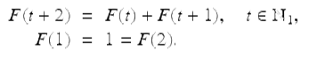
The Fibonacci sequence is given by
![]()
Fibonacci used this to model the population of pairs of rabbits under certain assumptions. To find F(t), note that F(t) is the solution of the IVP
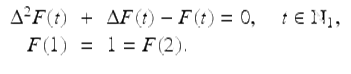
To solve this IVP we first get that the characteristic equation is
![]()
Hence, the characteristic values are
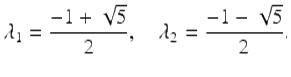
It follows that
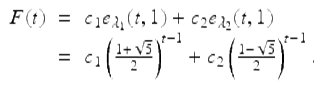
(1.17)
Applying the initial conditions we get the system
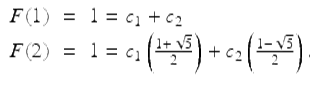
Solving this system for c 1 and c 2, using (1.17) and simplifying we get
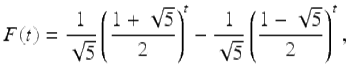
for ![]() Note F(t) is the integer nearest to
Note F(t) is the integer nearest to  . It follows that F(20) is the integer nearest
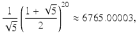
which gives us that F(20) = 6765.
Usually, we want to find all real-valued solutions of (1.13). When a characteristic root ![]() is complex,
is complex, ![]() is a complex-valued solution. In the next theorem we show how to use this complex-valued solution to find two linearly independent real-valued solutions on
is a complex-valued solution. In the next theorem we show how to use this complex-valued solution to find two linearly independent real-valued solutions on ![]() .
.
Theorem 1.33 (Complex Roots).
If the characteristic values are ![]() , β > 0 and α ≠ − 1, then a general solution of (1.13) is given by
, β > 0 and α ≠ − 1, then a general solution of (1.13) is given by
![]()
where ![]()
Proof.
First we show that if α ± i β, β > 0 are complex characteristic values of (1.13), then the condition p ≠ q + 1 is satisfied. In this case the characteristic equation for (1.13) is given by
![]()
It follows that p = −2α and q = α 2 +β 2. Therefore, 1 + q − p = (α + 1)2 +β 2 ≠ 0. This implies that p ≠ q + 1. By Theorem 1.31, we have that y(t) = e α+i β (t, a) is a complex-valued solution of (1.13). Using
we get that
![]()
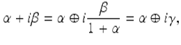
It follows from the (delta) Euler’s formula (1.11) that
![$$\displaystyle\begin{array}{rcl} y(t)& =& e_{\alpha }(t,a)e_{i\gamma }(t,a) {}\\ & =& e_{\alpha }(t,a)[\cos _{\gamma }(t,a) + i\sin _{\gamma }(t,a)] {}\\ & =& y_{1}(t) + iy_{2}(t) {}\\ \end{array}$$](fractional.files/image245.png)
is a solution of (1.13). But since p and q are real, we have that the real part, ![]() , and the imaginary part,
, and the imaginary part, ![]() , of y(t) are solutions of (1.13). Since p ≠ q + 1 and y 1(t), y 2(t) are linearly independent on
, of y(t) are solutions of (1.13). Since p ≠ q + 1 and y 1(t), y 2(t) are linearly independent on ![]() , we get from Remark 1.30 that
, we get from Remark 1.30 that
![]()
is a general solution of (1.13) on ![]() . □
. □
Example 1.34.
Solve the difference equation
![]()
(1.18)
The characteristic equation is
![]()
and so the characteristic values are ![]() . Hence using Theorem 1.33, we get
. Hence using Theorem 1.33, we get
![]()
is a general solution of (1.18) on ![]() .
.
The previous theorem (Theorem 1.33) excluded the case when the characteristic values of (1.13) are − 1 ± i β, where β > 0. The next theorem considers this case.
Theorem 1.35.
If the characteristic values of (1.13) are − 1 ± iβ, where β > 0, then a general solution of (1.13) is given by
![]()
![]()
Proof.
First note that by the first part of the proof of Theorem 1.33 we have that p ≠ q + 1. Since − 1 + i β is a characteristic root of (1.13), we have that y(t) = e −1+i β (t, a) is a complex-valued solution of (1.13). Now
![$$\displaystyle\begin{array}{rcl} y(t)& =& e_{-1+i\beta }(t,a) {}\\ & =& (i\beta )^{t-a} {}\\ & =& \left (\beta e^{i \frac{\pi }{2} }\right )^{t-a} {}\\ & =& \beta ^{t-a}\cos \left [ \frac{\pi } {2}(t - a)\right ] + i\beta ^{t-a}\sin \left [ \frac{\pi } {2}(t - a)\right ]. {}\\ \end{array}$$](fractional.files/image256.png)
It follows that
![]()
are solutions of (1.13). Since these solutions are linearly independent on ![]() , we have that
, we have that
![]()
is a general solution of (1.13). □
Example 1.36.
Solve the delta linear difference equation
![]()
The characteristic equation is ![]() , so the characteristic values are
, so the characteristic values are ![]() . It follows from Theorem 1.35 that
. It follows from Theorem 1.35 that
![]()
is a general solution on ![]()
Theorem 1.37 (Double Root).
Assume p ≠ 1 + q, and ![]() is a double root of the characteristic equation. Then
is a double root of the characteristic equation. Then
![]()
is a general solution of (1.13) .
Proof.
Since ![]() is a characteristic value, we have y 1(t) = e r (t, a) is a solution of (1.13). Since
is a characteristic value, we have y 1(t) = e r (t, a) is a solution of (1.13). Since ![]() , we have that the characteristic equation for (1.13) is
, we have that the characteristic equation for (1.13) is
![]()
Hence, in this case, (1.13) has the form
![]()
From Exercise 1.32, we have that y 2(t) = (t − a)e r (t, a) is a second solution of (1.13) on ![]() Since these two solutions are linearly independent on
Since these two solutions are linearly independent on ![]() , we have that
, we have that
![]()
is a general solution of (1.13). □
Example 1.38.
Evaluate the t by t determinant of the following tridiagonal matrix
![$$\displaystyle{M(t):= \left [\begin{array}{cccccccc} 4&4&0&0&\cdots &0&0&0\\ 1 &4 &4 &0 &\cdots &0 &0 &0 \\ 0&1&4&4&\cdots &0&0&0\\ 0 &0 &1 &4 &\cdots &0 &0 &0\\ \vdots & \vdots & \vdots & \vdots & \ddots & \vdots & \vdots & \vdots \\ 0&0&0&0&\cdots &4&4&0\\ 0 &0 &0 &0 &\cdots &1 &4 &4 \\ 0&0&0&0&\cdots &0&1&4 \end{array} \right ]}$$](fractional.files/image270.png)
for ![]() For example, we have that
For example, we have that
![$$\displaystyle{M(1):= \left [\begin{array}{*{10}c} 4 \end{array} \right ],\ M(2):= \left [\begin{array}{*{10}c} 4&4\\ 1 &4\\ \end{array} \right ],\ \text{and}\ \ M(3):= \left [\begin{array}{*{10}c} 4&4&0\\ 1 &4 &4 \\ 0&1&4\\ \end{array} \right ].}$$](fractional.files/image272.png)
Let D(t) be the value of the determinant of M(t). Expanding the t + 2 by t + 2 determinant D(t + 2) along its first row we get
![]()
Note that D(1) = 4 and D(2) = 12. It follows that if we define D(0) = 1, then we have
![]()
It then follows that D(t) is the solution of the IVP
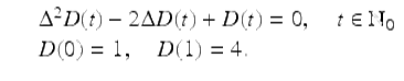
The characteristic equation is ![]() , and thus
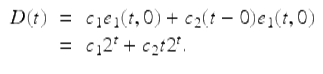
, and thus ![]() are the characteristic values. Hence by Theorem 1.37,
are the characteristic values. Hence by Theorem 1.37,
Using the initial conditions we get the system of equations
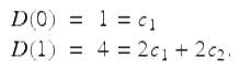
Solving this system we get that c 1 = c 2 = 1 and hence
![]()
The reader should check this answer for a few values of t.
Example 1.39.
Find the determinant D(t), ![]() of the t × t matrix that has zeros down the diagonal, 2’s down the superdiagonal, 8’s down the subdiagonal. This leads to solving the IVP
of the t × t matrix that has zeros down the diagonal, 2’s down the superdiagonal, 8’s down the subdiagonal. This leads to solving the IVP
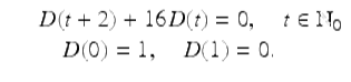
If we tried to use Theorem 1.33 to solve the difference equation D(t + 2) + 16D(t) = 0 we would write the equation D(t + 2) + 16D(t) = 0 in the form
![]()
The characteristic values for this equation are − 1 ± 4i. But Theorem 1.33 does not apply since the real part of − 1 ± 4i is − 1. Applying Theorem 1.44 we get that a general solution of D(t + 2) + 16D(t) = 0 is given by
![]()
Applying the initial conditions we get
![]()
for ![]()
Sometimes it is convenient to know how to solve the second order linear homogeneous difference equation when it is of the form
![]()
(1.19)
where ![]() and d ≠ 0 without first writing (1.19) (as we did in Examples 1.32 and 1.38) in the form (1.13). Exercise 1.36 shows that the difference equation 1.13 with p ≠ 1 + q is equivalent to the difference equation 1.19 with d≠ 0. Similar to the proof of Theorem 1.31 we can prove (Exercise 1.29) the theorem.
and d ≠ 0 without first writing (1.19) (as we did in Examples 1.32 and 1.38) in the form (1.13). Exercise 1.36 shows that the difference equation 1.13 with p ≠ 1 + q is equivalent to the difference equation 1.19 with d≠ 0. Similar to the proof of Theorem 1.31 we can prove (Exercise 1.29) the theorem.
Theorem 1.40 (Distinct Roots).
Assume d ≠ 0 and r 1 , r 2 are distinct roots of the equation
![]()
Then
![]()
is a general solution of (1.19) .
Example 1.41.
Solve the difference equation
![]()
(1.20)
Solving r 2 − 5r + 6 = (r − 2)(r − 3) = 0, we get r 1 = 2, r 2 = 3. It follows from Theorem 1.40 that
![]()
is a general solution of (1.20).
Similar to the proof of Theorem 1.37 one could prove (see Exercise 1.30) the following theorem.
Theorem 1.42 (Double Root).
Assume d ≠ 0 and r is a double root of r 2 + cr + d = 0. Then
![]()
is a general solution of (1.19) .
Example 1.43.
Solve the difference equation
![]()
(1.21)
Solving the equation r 2 + 4r + 4 = (r + 2)2 = 0, we get r 1 = r 2 = −2. It follows from Theorem 1.42 that
![]()
is a general solution of (1.21).
Theorem 1.44 (Complex Roots).
Assume d ≠ 0 and α ± iβ, β > 0 are complex roots of r 2 + cr + d = 0. Then
![]()
where ![]() and
and ![]() if α ≠ 0 and
if α ≠ 0 and ![]() if α = 0 is a general solution of (1.19) .
if α = 0 is a general solution of (1.19) .
Proof.
Since r = α + i β, β > 0 is a solution of r 2 + cr + d = 0, we have by Theorem 1.40 that y(t) = (α + i β) t is a (complex-valued) solution of (1.19). Let ![]() if α ≠ 0 and let
if α ≠ 0 and let ![]() if α = 0. Then if
if α = 0. Then if ![]() we have that
we have that
Since the real and imaginary parts of y(t) are linearly independent solutions of (1.19), we have that
![]()
is a general solution of (1.19). □
Next we briefly discuss the method of annihilators for solving certain nonhomogeneous difference equations. For an arbitrary function ![]() we define the operator E by
we define the operator E by
![]()
Then E n : = E ⋅ E n−1 for ![]() We say the polynomial in E,
We say the polynomial in E,
![]()
annihilates ![]() provided p(E)f(t) = 0 for
provided p(E)f(t) = 0 for ![]() Similarly we say the polynomial in the operator
Similarly we say the polynomial in the operator ![]() ,
,
![]()
annihilates ![]() provided
provided ![]()
Example 1.45.
Here are some simple annihilators for various functions:
(i)
(E − rI)r t = 0;
(ii)
![]()
(iii)
(E − rI)2 tr t = 0;
(iv)
![]()
(v)
![]()
(vi)
![]()
(vii)
![]()
(viii)
![]()
We now give some simple examples where we use the method of annihilators to solve various difference equations.
Example 1.46.
Solve the first order linear equation
![]()
(1.22)
First we write this equation in the form
![]()
Since E − 5I annihilates the right-hand side, we multiply each side by the operator E − 5I to get
![]()
It follows that a solution of (1.22) must be of the form
![]()
Substituting this into equation (1.22) we get
![]()
Hence we see that we must have ![]() . It follows that
. It follows that

is a general solution of (1.22).
Example 1.47.
Solve the second order linear nonhomogeneous difference equation
![]()
(1.23)
by the annihilator method. The difference equation (1.23) can be written in the form
![]()
Multiplying both sides by the operator E − 4I we get that
![]()
Hence y(t) must have the form
![]()
Substituting this into the difference equation (1.23) we get after simplification that 8c 3 = 16. Hence c 3 = 2 and we have that
![]()
is a general solution of (1.23).
Also we can use the method of annihilators to solve certain nonhomogeneous equations of the form
![]()
where p, q are real constants with p ≠ 1 + q, as is shown in the following example.
Example 1.48.
Use the method of annihilators to solve the nonhomogeneous equation
![]()
(1.24)
The equation (1.24) can be written in the form
![]()
Multiplying both sides by the operator ![]() we get that solutions of (1.24) are solutions of
we get that solutions of (1.24) are solutions of
![]()
The values of the characteristic equation ![]() are
are ![]()
![]()
![]() . Hence all solutions of (1.24) are of the form
. Hence all solutions of (1.24) are of the form
![]()
Substituting this into the equation we get that we must have 2c 3 e 3(t, a) = e 3(t, a) which gives us that c 3 = 2. Hence the general solution of (1.24) is given by
![]()