Discrete Fractional Calculus (2015)
1. Basic Difference Calculus
1.8. Second Order Linear Equations (Variable Coefficients)
In this section we will show how we can solve some second order linear equations (with possibly variable coefficients) by the method of factoring. As a special case of our factoring method we will solve Euler–Cauchy difference equations. We start with the following example to illustrate the method of factoring.
Example 1.71.
Solve the difference equation
![]()
(1.31)
The method we use to solve this equation is called the method of factoring. We first write our difference equation in the form
![]()
which also can be written in the factored form (using I as the identity operator)
![]()
Note that from Exercise 1.60 the operators ![]() and
and ![]() do not commute, so one has to be careful when one uses this method of factoring. Letting y(t) be a solution of our given difference equation and setting
do not commute, so one has to be careful when one uses this method of factoring. Letting y(t) be a solution of our given difference equation and setting ![]() , we get that
, we get that
![]()
which gives us the equation
![]()
By Theorem 1.14,
Since ![]() we have that
we have that
![]()
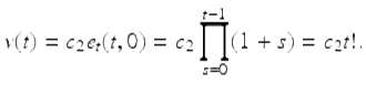
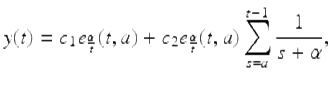
Using the variation of constants formula in Theorem 1.68, we get that
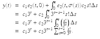
Hence
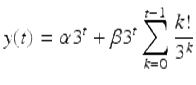
is a general solution of the difference equation (1.31).
We next show how we can use this method of factoring to solve the Euler–Cauchy difference equation
![]()
(1.32)
where c and d are real constants. We assume that
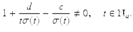
(1.33)
Since (1.33) holds, we have from Theorem 1.29 that solutions of IVPs for (1.32) are unique and solutions exist on ![]() . Also by Remark 1.30 we have that if y 1(t) and y 2(t) are linearly independent solutions of (1.32) on
. Also by Remark 1.30 we have that if y 1(t) and y 2(t) are linearly independent solutions of (1.32) on ![]() , then
, then
![]()
is a general solution of (1.32). We call the equation
![]()
(1.34)
or equivalently
![]()
(1.35)
the characteristic equation of the Euler–Cauchy difference equation (1.32) and the solutions of (1.34) and (1.35) the characteristic values (roots). Let α, β be the characteristic values, then the characteristic equation is given by
![]()
Hence
![]()
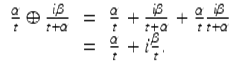
Note that
Hence we see that (1.33) holds if and only if
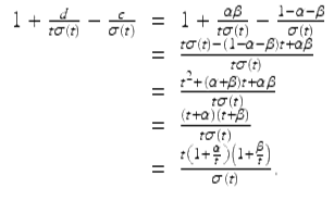
We now show how to factor the left-hand side of equation (1.32) assuming that (1.33) holds. Let ![]() Then, for
Then, for ![]() ,
,
![$$\displaystyle\begin{array}{rcl} & & t\sigma (t)\Delta ^{2}y(t) + ct\Delta y(t) + dy(t) {}\\ & & \quad = t\sigma (t)\Delta ^{2}y(t) + (1 -\alpha -\beta )t\Delta y(t) +\alpha \beta \; y(t) {}\\ & & \quad =\{ [t\sigma (t)\Delta ^{2}y(t) + t\Delta y(t)] -\beta t\Delta y(t)\} -\alpha [t\Delta y(t) -\beta y(t)] {}\\ & & \quad = t\Delta [t\Delta y(t) -\beta y(t)] -\alpha [t\Delta y(t) -\beta y(t)] {}\\ & & \quad = \left (t\Delta -\alpha I\right )\left (t\Delta -\beta I\right )y(t), {}\\ \end{array}$$](fractional.files/image504.png)
where I is the identity operator on the space of functions defined on ![]() . We call the difference equation
. We call the difference equation
![]()
(1.36)
the factored form of the Euler–Cauchy equation.
We will show that to solve the Euler–Cauchy equation we just need to find the characteristic values of (1.32). Next we solve the Euler–Cauchy equation by solving the factored form of the Euler–Cauchy equation (1.36).
Theorem 1.72 (Distinct Roots).
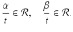
Assume α ≠ β are the characteristic values of the Euler–Cauchy difference equation (1.32) and ![]() . Then a general solution of the Euler–Cauchy equation (1.32) is given by
. Then a general solution of the Euler–Cauchy equation (1.32) is given by
![]()
for ![]()
Proof.
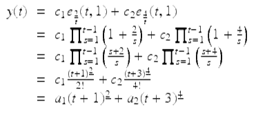
Note from the factored form of the Euler–Cauchy equation, if
![]()
then y(t) is a solution of the Euler–Cauchy equation (1.32). Since ![]() is a solution of
is a solution of
we have that ![]() is also a solution of (1.32). Now by Exercise 1.61, we can write the factored equation in the form
is also a solution of (1.32). Now by Exercise 1.61, we can write the factored equation in the form
![]()
Hence, by the above argument ![]() is a solution of (1.32). Since α ≠ β the solutions y 1(t), y 2(t) are linearly independent solutions on
is a solution of (1.32). Since α ≠ β the solutions y 1(t), y 2(t) are linearly independent solutions on ![]() . Hence a general solution of the Euler–Cauchy equation (1.32) is given by
. Hence a general solution of the Euler–Cauchy equation (1.32) is given by
![]()
for ![]() □
□
Example 1.73 (Distinct Real Roots).
Solve the Euler–Cauchy difference equation
![]()
(1.37)
The characteristic equation is
![]()
and so the characteristic values are r 1 = 2, r 2 = 4. It follows from Theorem 1.72 that a general solution of (1.37) is given by
for ![]()
Theorem 1.74 (Double Root).
Assume α is a double root of the characteristic equation for the Euler–Cauchy difference equation (1.32) and ![]() . Then a general solution of the Euler–Cauchy difference equation (1.32) is given by
. Then a general solution of the Euler–Cauchy difference equation (1.32) is given by
for ![]() .
.
Proof.
In this case the factored Euler–Cauchy equation is given by
![]()
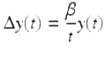
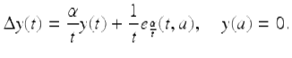
It follows that ![]() is a solution of this equation. To get a second solution note that by considering the factored equation we get that if y(t) satisfies the difference equation
is a solution of this equation. To get a second solution note that by considering the factored equation we get that if y(t) satisfies the difference equation
![]()
then y is a solution. In particular, let y 2 be the solution of the IVP
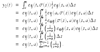
By the variation of constants formula in Theorem 1.68,
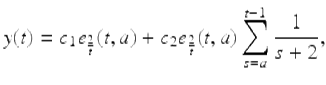
Since y 1(t), y 2(t) are linearly independent solutions of the given Euler–Cauchy equation we have that a general solution is given by
for ![]() □
□
Example 1.75 (Double Root).
Solve the Euler–Cauchy difference equation
![]()
(1.38)
where a > 0. The characteristic equation is given by
![]()
so 2 is a double root of the characteristic equation. By Theorem 1.74 we have that a general solution of (1.38) is given by
for ![]()
Theorem 1.76 (Complex Roots).
Assume r 1 = α + iβ, r 2 = α − iβ are the characteristic values of the Euler–Cauchy difference equation (1.32) and ![]() . Then a general solution of (1.32) is given by
. Then a general solution of (1.32) is given by
![]()
for ![]()
Proof.
By the proof of Theorem 1.72, we have that ![]() is a (complex-valued) solution of the Euler–Cauchy difference equation (1.32). Since
is a (complex-valued) solution of the Euler–Cauchy difference equation (1.32). Since ![]() it follows that
it follows that ![]() and hence
and hence ![]() is well defined on
is well defined on ![]() . Now consider
. Now consider
Using Euler’s formula (see Theorem 1.28, (vii) or Exercise 1.27), we have that
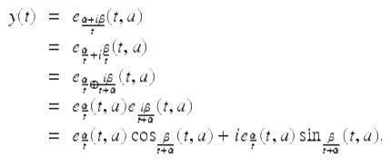
Since we are assuming the constants c, d in the Euler–Cauchy difference equation (1.32) are real, we have that
![]()
are real-valued solutions of the Euler–Cauchy difference equation (1.32). Since they are linearly independent on ![]() ,
,
![]()
is a general solution of the Euler–Cauchy difference equation (1.32). □
Example 1.77 (Complex Roots).
Solve the Euler–Cauchy difference equation
![]()
The characteristic equation is
![]()
and hence the characteristic values are r = 3 ± 2i. From Theorem 1.76, we get that
![]()
is a general solution.
For n ≥ 3 M. Bohner and E. Akin (see [63, Chapter 2]) defined the Euler–Cauchy difference equation of arbitrary order by
![]()
(1.39)
where we assume ![]() , 1 ≤ i ≤ n. For the reader interested in Euler–Cauchy difference equations of order n ≥ 3 see Exercise 1.67.
, 1 ≤ i ≤ n. For the reader interested in Euler–Cauchy difference equations of order n ≥ 3 see Exercise 1.67.