The history of mathematics: A brief course (2013)

Part VII. Special Topics

Chapter 36. Probability

One important part of modern mathematics that has not yet been mentioned is the theory of probability. Besides being a mathematical subject with its own special principles, it provides the mathematical apparatus for another discipline (statistics), which has perhaps more applications in the modern world than all of mathematics and also its own theoretical side. Unfortunately, we do not have space to discuss more than a few incidents in the history of statistics.

The word probability is related to the English words probe, probation, prove, and approve. All of these words originally had a sense of testing or experimenting,¹ reflecting their descent from the Latin probo, which has these meanings. In other languages the word used in this mathematical sense has a meaning more like plausibility,² as in the German Wahrscheinlichkeit (literally, truth resemblance) or the Russian veroyatnost' (literally, credibility, from the root ver-, meaning faith). The concept is very difficult to define in declarative sentences, precisely because it refers to phenomena that are normally described in the subjunctive mood. This mood has nearly disappeared in modern English; it clings to a precarious existence in the past tense, “If it were true that. . .” having replaced the older “If it be true that. . .”. The language of Aristotle and Plato, however, who were among the first people to discuss chance philosophically, had two such moods, the subjunctive and the optative, by which it was possible to express the difference between what would happen and what might happen. As a result, they could express more easily than we the intuitive concepts involved in discussing events that are imagined rather than observed.

Intuitively, probability attempts to express the relative strength of the feeling of confidence we have that an event will occur. How surprised would we be if the event happened? How surprised would we be if it did not happen? Because we do have different degrees of confidence in certain future events, quantitative concepts become applicable to the study of probability. Generally speaking, if an event occurs essentially all the time under specified conditions, such as an eclipse of the sun, we use a deterministic model (geometric astronomy, in this case) to study and predict it. If it occurs sometimes under conditions frequently associated with it, we rely on probabilistic models. Some earlier scientists and philosophers regarded probability as a measure of our

ignorance. Kepler, for example, believed that the supernova of 1604 in the constellation Serpent may have been caused by a random collision of particles; but in general he was a determinist who thought that our uncertainty about a roll of dice was merely a matter of insufficient data being available. He admitted, however, that he could find no law to explain the apparently random pattern of eccentricities in the elliptical orbits of the six planets known to him.

Once the mathematical subject got started, it developed a life of its own, in which theorems could be proved with the same rigor as in any other part of mathematics. Only the application of those theorems to the physical world remained and remains clouded by doubt. We use probability informally every day, as the weather forecast informs us that the chance of rain is 30% or 80% or 100%,³ or when we are told that one person in 30 will be afflicted with Alzheimer's disease between the ages of 65 and 74. Much of the public use of such probabilistic notions is, although not meaningless, at least of questionable value. For example, we are told that the life expectancy of an average American is now 77 years. Leaving aside the many assumptions of environmental and political stability used in the model that produced this number, we should at least ask one question: Can the number be related to the life of any person in any meaningful way? What plans can one base on it, since anyone may die on any given day, yet very few people can confidently rule out the possibility of living past age 90?⁴

The many uncertainties of everyday life, such as the weather and our health, occur mixed with so many possibly relevant variables that it would be difficult to distill a theory of probability from those intensely practical matters. What is needed is a simpler and more abstract model from which principles can be extracted and gradually made more sophisticated. The most obvious and accessible such models are games of chance. On them, probability can be given a quantitative and empirical formulation, based on the frequency of wins and losses. At the same time, the imagination can arrange the possible outcomes symmetrically and in many cases assign equal probabilities to different events. Finally, since money generally changes hands at the outcome of a game, the notion of a random variable (payoff to a given player, in this case) as a quantity assuming different values with different probabilities can be modeled.

36.1 Cardano

The mathematization of probability began in sixteenth-century Italy with Cardano. Todhunter (1865), on whose work the following discussion of Cardano's book is based, reports (p. 3) that Cardano gave the following table of values for a roll of three dice.

This table is enigmatic. Since it is impossible to roll a 1 with three dice, the first entry should perhaps be interpreted as the number of ways in which 1 may appear on at least one of the three dice. If so, then Cardan has got it wrong. One can imagine him thinking that if a 1 appears on one of the dice, the other two may show 36 different numbers, and since there are three dice on which the 1 may appear, the total number of ways of rolling a 1 must be 3 · 36 or 108. That way of counting ignores the fact that in some of these cases 1 appears on two of the dice or all three. By what is now known as the inclusion-exclusion principle, the total should be 3 · 36 − 3 · 6 + 1 = 91. But it is difficult to say what Cardano had in mind. The number 111 given for 2 may be the result of the same count, increased by the three ways of choosing two of the dice to show a 1. Todhunter worked out a simple formula giving these numbers, but could not imagine any gaming rules that would correspond to them. If indeed Cardano made mistakes in his computations, he was not the only great mathematician to do so.

Cardano's Liber de ludo (Book on Gambling) was published about a century after his death. In this book Cardano introduces the idea of assigning a probability p between 0 and 1 to an event whose outcome is not certain. The principal applications of this notion were in games of chance, where one might bet, for example, that a player could roll a 6 with one die given three chances. The subject is not developed in detail in Cardano's book, much of which is occupied by descriptions of the actual games played. Cardano does, however, state the multiplicative rule for a run of successes in independent trials. Thus the probability of getting a six on each of three successive rolls with one die is . Most important, he recognized the real-world application of what we call the law of large numbers, saying that when the probability for an event is p, then after a large number n of repetitions, the number of times it will occur does not lie far from the value np. This law says that it is not certain that the number of occurrences will be near np, but “that is where the smart money bets.”

36.2 Fermat and Pascal

After a bet has been made and before it is settled, a player cannot unilaterally withdraw from the bet and recover her or his stake. On the other hand, an accountant computing the net worth of one of the players ought to count part of the stake as an asset owned by that player; and perhaps the player would like the right to sell out and leave the game. What would be a fair price to charge someone for taking over the player's position? More generally, what happens if the game is interrupted? How are the stakes to be divided? The principle that seemed fair was that, regardless of the relative amount of the stake each player had bet, at each moment in the game a player should be considered as owning the portion of the stakes equal to that player's probability of winning at that moment. Thus, the net worth of each player is constantly changing as the game progresses, in accordance with what we now call conditional probability. Computing these probabilities in games of chance usually involves the combinatorial counting techniques the reader may have encountered in elementary discussions of probability. Problems of this kind were discussed in correspondence between Pascal and Fermat in the mid-seventeenth century.

A French nobleman, the Chevalier de Méré, who was fond of gambling, proposed to Pascal the problem of dividing the stakes in a game where one player has bet that a six will appear in eight rolls of a single die, but the game is terminated after three unsuccessful tries. Pascal wrote to Fermat that the player should be allowed to sell the throws one at a time. If the first throw is foregone, the player should take one-sixth of the stake, leaving five-sixths. Then if the second throw is also foregone, the player should take one-sixth of the remaining five-sixths or , and so on. In this way, Pascal argued that the fourth through eighth throws were worth .

This expression is the value of those throws before any throws have been made. If, after the bets are made but before any throws of the die have been made, the bet is changed and the players agree that only three throws shall be made, then the player holding the die should take this portion of the stakes as compensation for sacrificing the last five throws. Remember, however, that the net worth of a player is constantly changing as the game progresses and the probability of winning changes. The value of the fourth throw, for example, is smaller to begin with, since there is some chance that the player will win before it arrives, in which case it will not arrive. At the beginning of the game, the chance of winning on the fourth roll is . Here the factor in each term represents the probability that the player will not have won in the first k terms. After three unsuccessful throws, however, the probability that the player “will not have” won (that is to say, did not win) on the first three throws is 1, and so the probability of winning on the fourth throw becomes .

Fermat expressed the matter as follows:

[T]he three first throws having gained nothing for the player who holds the die, the total sum thus remaining at stake, he who holds the die and who agrees not to play his fourth throw should take as his reward. And if he has played four throws without finding the desired point and if they agree that he shall not play the fifth time, he will, nevertheless, have of the total for his share. Since the whole sum stays in play it not only follows from the theory, but it is indeed common sense that each throw should be of equal value.

Pascal wrote back to Fermat, proclaiming himself satisfied with Fermat's analysis and overjoyed to find that “the truth is the same at Toulouse and at Paris.”

36.3 Huygens

The Dutch mathematical physicist Christiaan Huygens (1629–1695), author of a very influential book on optics, wrote a treatise on probability in 1657. His De ratiociniis in ludo aleæ (On Reasoning in a Dice Game) consisted of 14 propositions and contained some of the results of Fermat and Pascal. In addition, Huygens considered multinomial problems, involving three or more players. Cardano's idea of an estimate of the expectation was elaborated by Huygens. He asserted, for example, that if there are p (equally likely) ways for a player to gain a and q ways to gain b, then the player's expectation is (pa + qb)/(p + q).

Even simple problems involving these notions can be subtle. For example, Huygens considered two players A and B taking turns rolling a pair of dice, with A going first. Any time A rolls a 6, A wins; any time B rolls a 7, B wins. What are the relative chances of winning? (The answer to that question would determine the fair proportions of the stakes to be borne by the two players.) Huygens concluded (correctly) that the odds were 31:30 in favor of B, that is, A's probability of winning was and B's probability was .

36.4 Leibniz

Although Leibniz wrote a full treatise on combinatorics, which provides the mathematical apparatus for computing many probabilities in games of chance, he did not himself gamble. But he did analyze many games of chance and suggest modifications of them that would make them fair (zero-sum) games. Some of his manuscripts on this topic have been analyzed by De Mora-Charles (1992). One of the games he analyzed is known as quinquenove. This game is played between two players using a pair of dice. One of the players, called the banker, rolls the dice, winning if the result is either a double or a total number of spots showing equal to 3 or 11. There are thus 10 equally likely ways for the banker to win with this roll, out of 36 equally likely outcomes. If the banker rolls a 5 or 9 (hence the name “quinquenove”), the other player wins. The other player has eight ways of winning of the equally likely 36 outcomes, leaving 18 ways for the game to end in a draw. The reader may be amused to learn that the great mathematician Leibniz, author of De arte combinatoria, confused permutations and combinations in his calculations for this game and got the probabilities wrong.

36.5 The Ars Conjectandi of James Bernoulli

One of the founding documents of probability theory was published in 1713, eight years after the death of its author, Leibniz’ disciple James Bernoulli. This work, Ars conjectandi (The Art of Prediction), moved probability theory beyond the limitations of analyzing games of chance. It was intended by its author to apply mathematical methods to the uncertainties of life. As he said in a letter to Leibniz, “I have now finished the major part of the book, but it still lacks the particular examples, the principles of the art of prediction that I teach how to apply to society, morals, and economics. . . .” That was an ambitious undertaking, and Bernoulli had not quite finished the work when he died in 1705.

Bernoulli noted an obvious gap between theory and application, saying that only in simple games such as dice could one apply the equal-likelihood approach of Huygens, Fermat and Pascal, whereas in the cases of practical importance, such as human health and longevity, no one had the power to construct a suitable model. He recommended statistical studies as the remedy to our ignorance, saying that if 200 people out of 300 of a given age and constitution were known to have died within 10 years, it was a 2-to-1 bet that any other person of that age and constitution would die within a decade.

In this treatise, Bernoulli reproduced the problems solved by Huygens and gave his own solution of them. He considered what are now called Bernoulli trials. These are repeated experiments in which a particular outcome either happens (success) with probability b/a or does not happen (failure) with probability c/a, the same probability each time the experiment is performed, each outcome being independent of all others. (A simple nontrivial example is rolling a single die, counting success as rolling a 3. Then the probabilities are and .) Since b/a + c/a = 1, Bernoulli saw that the binomial expansion would be useful in computing the probability of getting at least m successes in ntrials. He gave that probability as

It was, incidentally, in this treatise, when computing the sum of the rth powers of the first n integers, that Bernoulli introduced what are now called the Bernoulli numbers,⁵ defined by the formula

Nowadays we define these numbers as B₀ = 1, , and then , B₃ = 0, B₄ = B, and so forth. He illustrated his formula by finding

36.5.1 The Law of Large Numbers

Bernoulli imagined an urn containing numbers of black and white pebbles, whose ratio is to be determined by sampling with replacement. It is possible that you will always get a white pebble, no matter how many times you sample. However, if black pebbles constitute a significant proportion of the contents of the urn, this outcome is very unlikely. After discussing the degree of certainty that would suffice for practical purposes (he called it virtual certainty),⁶he noted that this degree of certainty could be attained empirically by taking a sufficiently large sample. The probability that the empirically determined ratio would be close to the true ratio increases as the sample size increases, but the result would be accurate only within certain limits of error, and

. . . we can attain any desired degree of probability that the ratio found by our many repeated observations will lie between these limits.

This last assertion is an informal statement of the law of large numbers for Bernoulli trials. If the probability of the outcome is p and the number of trials is n, this law can be phrased precisely by saying that for any ε > 0 there exists a number n₀ such that if m is the number of times the outcome occurs in n trials and n > n₀, the probability that the inequality |(m/n) − p| > ε will hold is less than ε.⁷ Bernoulli stated this principle in terms of the segment of the binomial series of (r + s)^n(r+s) consisting of the n terms on each side of the largest term (the term containing r^nrs^ns), and he proved it by giving an estimate on n sufficient to make the ratio of this sum to the sum of the remaining terms at least c, where c is specified in advance.

36.6 De Moivre

In 1711, even before the appearance of James Bernoulli's treatise, another ground-breaking book on probability appeared, the Doctrine of Chances, written by Abraham De Moivre (1667–1754), a French Huguenot who took refuge in England after 1685, when Louis XIV revoked the Edict of Nantes, issued by Henri IV to put an end to religious war in France by guaranteeing the civil rights of the Huguenots upon his accession to the throne in 1598.⁸ De Moivre's book went through several editions. Its second edition, which appeared in 1738, introduced a significant piece of numerical analysis, useful for approximating sums of terms of a binomial expansion (a + b)ⁿ for large n. De Moivre had published the work earlier in a paper written in 1733. Having no notation for the base e, which was introduced by Euler a few years later, De Moivre simply referred to the hyperbolic (natural) logarithm and “the number whose logarithm is 1.” De Moivre first considered only the middle term of the expansion. That is, for an even power n = 2m, he estimated the term

and found it equal to , where B was a constant for which he knew only an infinite series. At that point, he got stuck, as he admitted, until his friend James Stirling (1692–1770) showed him that “the Quantity B did denote the Square-root of the circumference of a circle whose Radius is Unity.”⁹ In our terms, , but De Moivre simply wrote c for B. Without having to know the exact value of B, De Moivre was able to show that “the Logarithm of the Ratio, which a Term distant from the middle by the Interval , has the the middle Term, is [approximately, for large n] .” In modern language,

De Moivre went on to say, “The Number, which answers to the Hyperbolic Logarithm −2 /n, [is]

By scaling, De Moivre was able to estimate segments of the binomial distribution. In particular, the fact that the numerator was ² and the denominator n allowed him to estimate the probability that the number of successes in Bernoulli trials would be between fixed limits. He came close to noticing that the natural unit of probability for n trials was a multiple of . In 1893, this natural unit of measure for probability was named the standard deviation by the British mathematician Karl Pearson (1857–1936). For Bernoulli trials with probability of success p at each trial the standard deviation is .

For what we would call a coin-tossing experiment in which —he imagined tossing a metal disk painted white on one side and black on the other—de Moivre observed that with 3600 coin tosses, the odds would be more than 2 to 1 against a deviation of more than 30 “heads” from the expected number of 1800. The standard deviation for this experiment is exactly 30, and 68 percent of the area under a normal curve lies within one standard deviation of the mean. De Moivre could imagine the bell-shaped normal curve that we are familiar with, but he did not give it the equation it now has (). Instead he described it as the curve whose ordinates were numbers having certain logarithms. What seems most advanced in his analysis is that he recognized the area under the curve as a probability and computed it by a mechanical quadrature method that he credited jointly to Newton, Roger Cotes, James Stirling, and himself. This tendency of the distribution density of the average of many independent, identically distributed random variables to look like the bell-shaped curve is called the central limit theorem.

36.7 The Petersburg Paradox

Soon after its introduction by Huygens and James Bernoulli the concept of mathematical expectation came in for some critical appraisal. While working in the Russian Academy of Sciences, Daniel Bernoulli discussed the problem now known as the Petersburg paradox with his brother Nicholas (1695–1726, known as Nicholas II). We can describe this paradox informally as follows. Suppose that you toss a coin until heads appears. If it appears on the first toss, you win $2, if it first appears on the second toss, you win $4, and so on; if heads first appears on the nth toss, you win 2ⁿ dollars. How much money would you be willing to pay to play this game? Now by “rational” computations the expected winning is infinite, being , so that you should be willing to pay, say, $10,000 to play each time. On the other hand, who would bet $10,000 knowing that there was an even chance of winning back only $2, and that the odds are 7 to 1 against winning more than $10? Something more than mere expectation was involved here.

Daniel Bernoulli discussed the matter at length in an article in the Commentarii of the Petersburg Academy for 1730–1731 (published in 1738). He argued for the importance of something that we now call utility. If you already possess an amount of money x and you receive a small additional amount of money dx, how much utility does the additional money have for you, subjectively? Bernoulli assumed that the increment of utility dy was directly proportional to dx and inversely proportional to x, so that

and as a result, the total utility of personal wealth is a logarithmic function of total wealth.

One consequence of this assumption is a law of diminishing returns: The additional satisfaction from additional wealth decreases as wealth increases. Bernoulli used this idea to explain why a rational person would refuse to play the game. Obviously, the expected gain in utility from each of these wins, being proportional to the logarithm of the money gained, has a finite total, and so one should be willing to pay only an amount of money that has an equal utility to the gambler. A different explanation, which seems to have been given first by the mathematician John Venn (1834–1923) of Caius¹⁰ College, Cambridge in 1866, invokes the decreasing marginal utility of gain versus risk to explain why a rational person would not pay a large sum to play this game.

The utility y, which Bernoulli called the emolumentum (gain), is an important tool in economic analysis, since it provides a dynamic model of economic sellers exchange goods and services for money of higher personal utility. If money, goods, and services did not have different utility for different people, no market could exist at all.¹¹ That idea is valid independently of the actual formula for utility given by Bernoulli, although, as far as measurements of pyschological phenomena can be made, Bernoulli's assumption was extremely good. The physiologist Ernst Heinrich Weber (1795–1878) asked blindfolded subjects to hold weights, which he gradually increased, and to say when they noticed an increase in the weight. He found that the threshold for a noticeable difference was indeed inversely proportional to the weight. That is, if S is the perceived weight and W the actual weight, then dS = k dW/W, where dW is the smallest increment that can be noticed and dS the corresponding perceived increment. Thus he found exactly the law assumed by Bernoulli for perceived increases in wealth.¹² Utility is of vital importance to the insurance industry, which makes its profit by having a large enough stake to play “games” that resemble the Petersburg paradox.

One important concept was missing from the explanation of the Petersburg paradox. Granted that one should expect the “expected” value of a quantity depending on chance, how confidently should one expect it? The question of dispersion or variance of a random quantity lies beneath the surface here and needed to be brought out. (Variance is the square of the standard deviation.) It turns out that when the expected value is infinite, or even when the variance is infinite, no rational projections can be made. Since we live in a world of finite duration and finite resources, however, each game will be played only a finite number of times. It follows that every actual game has a finite expectation and variance and is subject to rational analysis using them.

36.8 Laplace

Although Pierre-Simon Laplace (1749–1827) is known primarily as an astronomer, he also developed a great deal of theoretical physics. (The partial differential equation satisfied by harmonic functions is named after him.) He also understood the importance of probabilistic methods in the analysis of data. In his Théorie analytique des probabilités, he proved that the distribution of the average of random observational errors that are uniformly distributed in an interval symmetric about zero tends to the normal distribution as the number of observations increases. Except for using the letter c where we now use e to denote the base of natural logarithms, he had what we now call the central limit theorem for independent uniformly distributed random variables.

36.9 Legendre

In a treatise on methods of determining the orbits of comets, published in 1805, Legendre dealt with the problem that frequently results when observation meets theory. Theory prescribes a certain number of equations of a particular form to be satisfied by the observed quantities. These equations involve certain parameters that are not observed, but are to be determined by fitting observations to the theoretical model. Observation provides a large number of empirical, approximate solutions to these equations, and thus normally provides a number of equations far in excess of the number of parameters to be chosen. If the law is supposed to be represented by a straight line, for example, only two constants are to be chosen. But the observed data will normally not lie on a line; instead, they may cluster around a line. How is the observer to choose canonical values for the parameters from the observed values of each of the quantities?

Legendre's solution to this problem is now a familiar technique. If the theoretical equation is y = f(x), where f(x) involves parameters α, β,. . ., and one has data points (x_k, y_k), k = 1,. . ., n, sum the squares of the “errors” f(x_k) − y_k to get an expression in the parameters

and then choose the parameters so as to minimize E. For fitting with a straight line y = ax + b, for example, one needs to choose E(a, b) given by

so that

36.10 Gauss

Legendre was not the first to study the problem of determining the most likely value of a quantity x using the results of repeated measurements of it, say x_k, k = 1,. . ., n. In 1799 Laplace had tried the technique of taking the value xthat minimizes the sum of the absolute errors¹³ |x − x_k|. But still earlier, in 1794 as shown by his diary and correspondence, the teenager Gauss had hit on the least-squares technique for the same purpose. As Reich (1977, p. 56) points out, Gauss did not consider this discovery very important and did not publish it until 1809. In 1816, Gauss published a paper on observational errors, in which he discussed the most probable value of a variable based on a number of observations of it. His discussion was much more modern in its notation than those that had gone before, and also much more rigorous. He found the likelihood of an error of size x to be

where h was what he called the measure of precision. He showed how to estimate this parameter by inverse-probability methods. In modern terms, , where σ is the standard deviation. This work brought the normal distribution into a standard form, and it is now often referred to as the Gaussian distribution.

36.11 Philosophical Issues

The notions of chance and necessity have often played a role in philosophical speculation; in fact, most books on logic are kept in the philosophy sections of libraries. Many of the mathematicians who have worked in this area have had a strong interest in philosophy and have speculated on what probability means. In so doing, they have come up against the same difficulties that confront natural philosophers when trying to explain how induction works. Like Pavlov's dogs and Skinner's pigeons (see Chapter 1), human beings tend to form expectations based on frequent, but not necessarily invariable conjunctions of events and seem to find it very difficult to suspend judgment and live with no belief where there is no evidence.¹⁴ Can philosophy offer us any assurance that proceeding by induction based on probability and statistics is any better than, say, divination? Are insurance companies acting on pure faithwhen they offer to bet us that we will survive long enough to pay them more money (counting the return on investment) in life insurance premiums than they will pay out when we die? If probability is a subjective matter, is subjectivity the same as arbitrariness?

What is probability, when applied to the physical world? Is it merely a matter of frequency of observation, and consequently objective? Or do human beings have some innate faculty for assigning probabilities? For example, when we toss a coin twice, there are four distinguishable outcomes: HH, HT, TH, TT. Are these four equally likely? If one does not know the order of the tosses, only three possibilities can be distinguished: two heads, two tails, and one of each. Should those be regarded as equally likely, or should we imagine that we do know the order and distinguish all four possibilities?¹⁵ Philosophers still argue over such matters. Siméon-Denis Poisson (1781–1840) seemed to be having it both ways in his Recherches sur la probabilité des jugemens (Investigations into the Plausibility of Inferences) when he wrote that

The probability of an event is the reason we have to believe that it has taken place, or that it will take place.

and then immediately followed up with this:

The measure of the probability of an event is the ratio of the number of cases favorable to that event, to the total number of cases favorable or contrary.

In the first statement, he appeared to be defining probability as a subjective event, one's own personal reason, but then proceeded to make that reason an objective thing by assuming equal likelihood of all outcomes. Without some restriction on the universe of discourse, these definitions are not very useful. We do not know, for example, whether our automobile will start tomorrow morning or not, but if the probability of its doing so were really only 50% because there are precisely two possible outcomes, most of us would not bother to buy an automobile. Surely Poisson was assuming some kind of symmetry that would allow the imagination to assign equal likelihoods to the outcomes, and intending the theory to be applied only in those cases. Still, in the presence of ignorance of causes, equal probabilities seem to be a reasonable starting point. The law of entropy in thermodynamics, for example, can be deduced as a tendency for an isolated system to evolve to a state of maximum probability, and maximum probability means the maximum number of equally likely states for each particle.

36.12 Large Numbers and Limit Theorems

The idea of the law of large numbers was stated imprecisely by Cardano and with more precision by James Bernoulli. To better carry out the computations involved in using it, De Moivre was led to approximate the binomial distribution with what we now realize was the normal distribution. He, Laplace, and Gauss all grasped with different degrees of clarity the principle (central limit theorem) that when independent measurements are averaged, their distribution density tends to resemble the bell-shaped curve.

The law of large numbers was given its name in the 1837 work of Poisson just mentioned. Poisson discovered an approximation to the probability of getting at most k successes in n trials, valid when n is large and the probability pis small. He thereby introduced what is now known as the Poisson distribution, in which the probability of k successes is given by

The Russian mathematician Chebyshëv¹⁶ (1821–1894) introduced the concept of a random variable and its mathematical expectation. He is best known for his 1846 proof of the weak law of large numbers for repeated independent trials. That is, he showed that the probability that the actual proportion of successes will differ from the expected proportion by less than any specified ε > 0 tends to 1 as the number of trials increases. In 1867 he proved what is now called Chebyshëv's inequality: The probability that a random variable will assume a value more than [what is now called k standard deviations] from its mean is at most 1/k². This inequality was published by Chebyshëv's friend and translator Irénée-Jules Bienaymé (1796–1878) and is sometimes called the Chebyshëv–Bienaymé inequality (see Heyde and Seneta, 1977). This inequality implies the weak law of large numbers. In 1887, Chebyshëv also stated the central limit theorem for independent random variables.

The extension of the law of large numbers to dependent trials was achieved by Chebyshëv's student Andrei Andreevich Markov (1856–1922). The subject of dependent trials—known as Markov chains—remains an object of current research. In its simplest form it applies to a system in one of a number of states {S₁,. . ., S_n} which at specified times may change from one state to another. If the probability of a transition from S_i to S_j is p_ij, the matrix

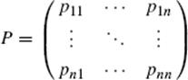
is called the transition matrix. If the transition probabilities are the same at each stage, one can easily verify that the matrix power P^k gives the probabilities of the transitions in k steps.

Problems and Questions

Mathematical Problems

36.1 We saw above that Cardano (probably) and Pascal and Leibniz (certainly) miscalculated some elementary probabilities. As an illustration of the counterintuitive nature of many simple probabilities, consider the following hypothetical games. (A casino could probably be persuaded to provide these games if there was enough public interest in them.) In Game 1 the dealer draws two randomly chosen cards from a deck on the table and looks at them. If neither card is an ace, the dealer shows them to the other players, and no game is played. The cards are replaced in the deck, the deck is shuffled, and the game begins again. If one card is an ace, players are not shown the cards, but are invited to bet against a fixed winning amount offered by the house that the other card is also an ace. What winning should the house offer (in order to break even in the long run) if players pay one dollar per bet?

In Game 2 the rules are the same, except that the game is played only when one of the two cards is the ace of hearts. What winning should the house offer in order to break even charging one dollar to bet? Why is this amount not the same as for Game 1?

36.2 Use the Maclaurin series for to verify that the series given by De Moivre, which was

represents the integral

which is the area under a standard normal (bell-shaped) curve above the mean, but by at most one standard deviation, as given in many tables.

36.3 Radium-228 is an unstable isotope. Each atom of Ra-228 has a probability of 0.1145 (about 1 chance in 9, or about the probability of rolling a 5 with two dice) of decaying to form an atom of actinium within any given year. This means that the probability that the atom will survive the year as an atom of Ra-228 is 1 − 0.1145 = 0.8855. Denote this “one-year survival” probability by p. Because any sample of reasonable size contains a huge number of atoms, that survival probability (0.8855) is the proportion of the weight of Ra-228 that we would expect to survive a year.

If you had one gram of Ra-228 to begin with, after one year you would expect to have p = 0.8855 grams. Each succeeding year, the weight of the Ra-228 left would be multiplied by p, so that after two years you would expect to have p² = (0.8855)² = 0.7841 grams. In general, after t years, if you started with W₀ grams, you would expect to have W = W₀p^t grams. Now push these considerations a little further and determine how strongly you can rely on this expectation. Recall Chebyshëv's inequality, which says that the probability of being more than k standard deviations from the expected value is never larger than (1/k)². What we need to know to answer the question in this case is the standard deviation σ.

Assume that each atom decays at random, independently of what happens to any other atom. This independence allows us to think that observing our sample for a year amounts to a large number of “independent trials,” one for each atom. We test each atom to see if it survived as an Ra-228 atom or decayed into actinium. Let N₀ be the number of atoms that we started with. Assuming that we started with 1 gram of Ra-228, there will be N₀ = 2.642 · 10²¹atoms of Ra-228 in the original sample.¹⁷ That is a very large number of atoms. The survival probability is p = 0.8855. For this kind of independent trial, as mentioned the standard deviation with N₀ trials is

We write the standard deviation in this odd-looking way so that we can express it as a fraction of the number N₀ that we started with. Since weights are proportional to the number of atoms, that same fraction will apply to the weights as well.

Put in the given values of p and N₀ to compute the fraction of the initial sample that constitutes one standard deviation. Since the original sample was assumed to be one gram, you can regard the answer as being expressed in grams. Then use Chebyshëv's inequality to estimate the probability that the amount of the sample remaining will differ from the theoretically predicted amount by 1 millionth of a gram (1 microgram, that is, 10⁻⁶ grams)? [Hint: How many standard deviations is one millionth of a gram?]

Historical Questions

36.4 From what real-life situations did the first mathematical analyses of probability arise?

36.5 What new concepts were introduced in James Bernoulli's Ars conjectandi?

36.6 What are the two best-known mathematical theorems about the probable outcome of a large number of random trials?

Questions for Reflection

36.7 Consider the case of 200 men and 200 women applying to a university consisting of only two different departments, and assume that the acceptance rates are given by the following table.

Observe that the admission rate for men in department A is , while that for women is . In department B the admission rate for men is and for women it is . In both cases, the people making the admission decisions are admitting a higher proportion of women than of men. Yet the overall admission rate is 64% for men and only 36% for women. Explain this paradox in simple, nonmathematical language.

This paradox was first pointed out by George Udny Yule (1871–1951) in 1903. Yule produced a set of two 2 × 2 tables, each of which had no correlation, but produced a correlation when combined (see David and Edwards, 2001, p. 137). Yule's result was, for some reason, not given his name; but because it was publicized by Edward Hugh Simpson in 1951,¹⁸ it came to be known as Simpson's paradox.¹⁹ Simpson's paradox is a counterintuitive oddity, not a contradiction.

An example of it occurred in the admissions data from the graduate school of the University of California at Berkeley in 1973. These data raised some warning flags. Of the 12,763 applicants, 5232 were admitted, giving an admission rate of 41%. However, investigation revealed that 44% of the male applicants had been admitted and only 35% of the female applicants. There were 8442 male applicants, 3738 of whom were accepted, and 4321 female applicants, 1494 of whom were accepted. Simple chi-square testing showed that the hypothesis that these numbers represent a random deviation from a sex-independent acceptance rate of 41% was not plausible. There was unquestionably bias. The question was: Did this bias amount to discrimination? If so, who was doing the discriminating?

For more information on this case study and a very surprising conclusion, see “Sex bias in graduate admissions: Data from Berkeley,” Science, 187, 7 February 1975, 398–404. In that paper, the authors analyzed the very evident bias in admissions to look for evidence of discrimination. Since admission decisions are made by the individual departments, it seemed logical to determine which departments had a noticeably higher admission rate for men than for women. Surprisingly, the authors found only four such departments (out of 101), and the imbalance resulting from those four departments was more than offset by six other departments that had a higher admission rate for women.

36.8 It is interesting that an exponential law of growth or decay can be associated with both completely deterministic models of growth (compound interest) and completely random models, as in the case of radioactive decay. Is it possible to assume physical laws that would make radioactive decay completely deterministic?

36.9 In the Power Ball lottery that is played by millions of people in the United States every week, players are trying to guess which five of 59 numbered balls will drop out of a hopper, and which one of 39 others will drop out of a hopper. The jackpot is won by guessing all six correctly. Any combination of 5 numbers and 1 number is as likely to drop as any other. Hence, the number of possible combinations is

This is, needless to say, a rather large number, meaning that the odds are heavily against the player. To picture the odds more vividly, imagine that the winning combinations are the serial numbers on dollar bills, and that this $195,249,054 consists of one-dollar bills laid end to end. They would cover more than 30,000 km, roughly the distance from the North Pole to the South Pole and then north again to the Equator. Even if the journey could all be made on level ground, it would require a vigorous walker 250 days to make it with no stops to rest. In that scenario, the gambler is going to bend down just once and hope to pick up the winning dollar bill.

Still, somebody does eventually win the Power Ball, every few weeks or months. Why is this fact not surprising? Is it a rational wager to spend a dollar to play the lottery if the prize goes above this stake, on the grounds that the expected gain is larger than the cost of playing?

Notes

1. The common phrase “the exception that proves the rule” is nowadays misunderstood and misused because of this shift in the meaning of the word prove. Exceptions test rules, they do not prove them in the current sense of that word. In fact, quite to the contrary, exceptions disprove rules.

2. Here is another interesting word etymology. The root is plaudo, meaning strike, but specifically meaning to clap one's hands together, to applaud. Once again, approval is involved in the notion of probability.

3. These numbers are generated by computer models of weather patterns for squares in a grid representing a geographical area. The modeling of their accuracy also uses probabilistic notions.

4. The Russian mathematician Yu. V. Chaikovskii (2001) believes that some of this cloudiness is about to be removed with the creation of a new science he calls aleatics (from the Latin word alea, meaning dice-play or gambling). We must wait and see. A century ago, other Russian mathematicians confidently predicted a bright future for arithmology.

5. As mentioned in Chapter 24, a table of these numbers can be found in Seki Kwa's posthumously published Katsuy Samp, which appeared the year before Bernoulli's work.

6. This phrase is often translated more literally as moral certainty, which has the wrong connotation.

7. Probabilists say that the frequency of successes converges “in probability” to the probability of success at each trial. Analysts say it converges “in measure.” There is also a strong law of large numbers, more easily stated in terms of independent random variables, which asserts that (under suitable hypotheses) there is a set of probability 1 on which the convergence to the mean occurs. That is, the convergence is “almost surely,” as probabilists say, and “almost everywhere,” as analysts phrase the matter. On a finite measure space such as a probability space, almost everywhere convergence implies convergence in measure, but the converse is not true.

8. The spirit of sectarianism has infected historians to the extent that Catholic and Protestant biographers of De Moivre do not agree on how long he was imprisoned in France for being a Protestant. They do agree that he was imprisoned, however. To be fair to the French, they did elect him a member of the Academy of Sciences a few months before his death.

9. The approximation is now called Stirling's formula.

10. Pronounced “Keys.”

11. One feels the lack of this concept very strongly in the writing on economics by Aristotle and his followers, especially in their condemnation of the practice of lending money at interest, which ignores the utility of time.

12. Weber's result was publicized by Gustave Theodor Fechner (1801–1887) and is now known as the Weber–Fechner law.

13. This method has the disadvantage that one large error and many small errors count equally. The least-squares technique avoids that problem.

14. In his Formal Logic, Augustus De Morgan imagined asking a person selected at random for an opinion whether the volcanoes—he meant craters—on the unseen side of the moon were larger than those on the side we can see. He concluded, “The odds are, that though he has never thought of the question, he has a pretty stiff opinion in three seconds.”

15. If the answer to that question seems intuitively obvious, please note that in more exotic applications of statistics, such as in quantum mechanics, either possibility can occur. Fermions have wave functions that are antisymmetric, and they distinguish between HT and TH; bosons have symmetric wave functions and do not distinguish them.

16. Properly pronounced “Cheb-wee-SHAWF,” but more commonly “CHEB-ee-shev,” by English speakers.

17. The number of atoms in one gram of Ra-228 is the Avogadro number 6.023 · 10²³ divided by 228.

18. See “The interpretation of interaction in contingency tables,” Journal of the Royal Statistical Society, Series B, 13, 238–241.

19. The name Simpson's paradox goes back at least to the article of C. R. Blyth, “On Simpson's paradox and the sure-thing principle,” in the Journal of the American Statistical Association, 67 (1972), 364–366.