The history of mathematics: A brief course (2013)

Part VII. Special Topics

Chapter 41. Complex Analysis

In the mid-1960s, the late Walter Rudin (1921–2010), the author of several standard graduate textbooks in mathematics, wrote a textbook with the title Real and Complex Analysis, aimed at showing the considerable unity and overlap between the two subjects. It was necessary to write such a book because real and complex analysis, while sharing common roots in the calculus, had developed quite differently. The contrasts between the two are considerable. Complex analysis considers the smoothest, most orderly possible functions, those that are analytic, while real analysis allows the most chaotic imaginable functions. Complex analysis was, to pursue our botanical analogy, fully a “branch” of calculus, and foundational questions hardly entered into it. Real analysis had a share in both roots and branches, and it was intimately involved in the debate over the foundations of calculus.

What caused the two varieties of analysis to become so different? Both deal with functions, and both evolved under the stimulus of the differential equations of mathematical physics. The central point is the concept of a function. We have already seen the early definitions of this concept by Leibniz and John Bernoulli. All mathematicians from the seventeenth and eighteenth centuries had an intuitive picture of a function as a formula or expression in which variables are connected by rules derived from algebra or geometry. A function was regarded as continuous if it was given by a single formula throughout its range. If the formula changed, the function was called “mechanical” by Euler. Although “mechanical” functions may be continuous in the modern sense, they are not usually analytic. All the “continuous” functions in the older sense are analytic. They have power-series expansions, and those power-series expansions are often sufficient to solve differential equations. As a general signpost indicating where the paths diverge, the path of power-series expansions and the path of trigonometric-series expansions is a rough guide. A consequence of the development was that real-variable theory had to deal with very irregular and “badly behaved” functions. It was therefore in real analysis that the delicate foundational questions arose. This chapter and the two following are devoted to exploring these developments.

41.1 Imaginary and Complex Numbers

Although imaginary numbers seem more abstract to modern mathematicians than negative and irrational numbers, that is because their physical interpretation is more remote from everyday experience. One interpretation of , for example, is as a rotation through a right angle. (Since i² = − 1, the effect of multiplying a real number twice by i is to rotate the real axis by 180. Hence multiplying once by i ought to rotate it by 90.)

We have an intuitive picture of the length of a line segment and decimal approximations to describe that length as a number; that is what gives us confidence that irrational numbers really are numbers. But it is difficult to think of a rotation as a number. On the other hand, the rules for multiplying complex numbers—at least those whose real and imaginary parts are rational—are much simpler and easier to understand than the definition of irrational numbers. In fact, complex numbers were understood before real numbers were properly defined; mathematicians began trying to make sense of them as soon as there was a clear need to do so. That need came not, as one might expect, from trying to solve quadratic equations such as x² − 2x + 2 = 0, where the quadratic formula produces . It was possible in this case simply to say that the equation had no solution.

To find the origin of imaginary numbers, we need to return to the algebraic solution of cubic equations that we discussed in Chapters 30 and 37. Recall that the algorithm for finding the solution had the peculiar property that it involved taking the square root of a negative number precisely when there were three distinct real solutions. For example, the algorithm gives the solution of x³ − 7x + 6 = 0 as

We cannot say that the equation has no roots, since it obviously has 1, 2, and −3 as roots. Thus the challenge arose: Make sense of this formula. Make it say “1, 2, and −3.”

This challenge was taken up by Bombelli, who wrote a treatise on algebra which he wrote in 1560, but which was not published until 1572. In that treatise he invented the name “plus of minus” to denote a square root of −1 and “minus of minus” for its negative. He did not think of these two concepts as different numbers, but rather as the same number being added in the first case and subtracted in the second. What is most important is that he realized what rules must apply to them in computation: plus of minus times plus of minus makes minus and minus of minus times minus of minus makes minus, while plus of minus times minus of minus makes plus. Bombelli had an ad hocmethod of taking the cube root of a complex number, opportunistically taking advantage of any extra symmetry in the number whose root was to be extracted. In considering the equation x³ = 15x + 4, for example, he found by applying the formula that . In this case, however, Bombelli was able to work backward, since he knew in advance that one root is 4; the problem was to make the formula say “4.” Bombelli had the idea that the two cube roots must consist of real numbers together with his “plus of minus” or “minus of minus.” Since the numbers under the cube root sign are (as we would say) complex conjugates of each other, it would seem likely that the two cube roots are as well. That is the real parts are equal, and the imaginary parts are negatives of each other. Since the sum of the two cube roots is four, it follows that the real parts must be 2. Thus . The number t is now easily found by cubing: . Obviously, t = 1, and so . If we didn't know a root, this approach would lead nowhere; but if a solution is given, it explains how the imaginary numbers are to be interpreted and used in computation.

41.1.1 Wallis

In an attempt to make these numbers more familiar, the English mathematician John Wallis (1616–1703) pointed out that while no positive or negative number could have a negative square, nevertheless it is also true that no physical quantity can be negative, that is, less than nothing. Yet negative numbers were accepted and interpreted as retreats when the numbers measure advances along a line. Wallis thought that what was allowed in lines might also apply to areas, pointing out that if 30 acres are reclaimed from the sea, and 40 acres are flooded, the net amount “gained” from the sea would be −10 acres. Although he did not say so, it appears that he regarded this real loss of 10 acres as an imaginary gain of a square of land feet on a side.

What he did say in his 1673 treatise on algebra was that one could represent as the mean proportional between a and −b. The mean proportional is easily found for two positive line segments a and b. Simply lay them end to end, use the union as the diameter of a circle, and draw the half-chord perpendicular to that diameter at the point where the two segments meet. That half-chord (sine) is the mean proportional. If only mathematicians had used the Euclidean construction of the mean proportional, interpreting points to the left of 0 as negative, they would have gotten the geometric interpretation of imaginary numbers as points on an axis perpendicular to the real numbers, as shown in the drawing on the left in Fig. 41.1.

Figure 41.1 (1) How it might have been: The mean proportional between a positive number a and a negative number −b lies on an axis perpendicular to them. (2) How Wallis thought of it: The mean proportional is a tangent instead of a sine.

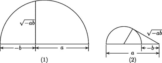
As things turned out, however, this idea took some time to catch on. Wallis' thinking went in a different direction. When one of the numbers was regarded as negative, he regarded the negative quantity as an oppositely directed line segment. He then modified the construction of the mean proportional between the two segments. When two oppositely directed line segments are joined end to end, one end of the shorter segment lies between the point where the two segments meet and the other end of the longer segment, so that the point where the segments join up lies outside the circle passing through their other two endpoints. Wallis interpreted the mean proportional as the tangent to the circle from the point where the two segments meet. Thus, whereas the mean proportional between two positive quantities is represented as a sine, that between a positive and negative quantity is represented as a tangent. This approach is quite consistent, since the endpoint of b can move in either direction without upsetting the numerical relationship between the lines. And indeed, it is easy to verify that the length of Wallis' tangent line is indeed the mean proportional between the lengths of the two given lines.

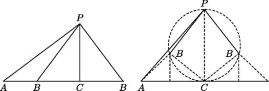
Wallis applied this procedure in an “imaginary” construction problem. First he stated the following “real” problem. Given a triangle having side AP of length 20, side PB of length 15, and altitude PC of length 12, find the length of side AB, taken as base in Fig. 41.2. Wallis pointed out that two solutions were possible. Using the foot of the altitude as the reference point C and applying the Pythagorean theorem twice, he found that the possible lengths of ABwere 16 ± 9, that is, 7 and 25. (In general .) He then proposed reversing the data, in effect considering an impossible triangle having side AP of length 20, side PB of length 12, and altitude PC of length 15. The two solutions would thus appear to be . Although the algebraic problem has no real solution, a fact verified by the geometric figure (Fig. 41.1), one could certainly draw the two line segments AB. These line segments could therefore be interpreted as the numerical solutions of the equation, representing a triangle with one side (AB) having imaginary (actually complex) length: AB = AC ± BC. In the figure , and so the two sides drawn as BC (which really do have length 9) represent . Once again, the imaginary part of the representation is oblique to the real part, but not perpendicular to it.

Figure 41.2 Wallis' geometric solution of quadratic equation with real roots (left) and complex roots (right).

The rules given by Bombelli had made imaginary and complex numbers accessible, and they turned out to be very convenient in many formulas. Euler made free use of them, studying power series in which the variables were allowed to be complex numbers and deriving a famous formula

Euler derived this result in a paper on ballistics written around 1727 (see Smith, 1929, pp. 95–98), just after he moved to Russia. He had no thought of representing as we now do, on a line perpendicular to the real axis.

41.1.2 Wessel

Wallis' work had given the first indication that complex numbers would have to be interpreted as line segments in a plane, a discovery made again 70 years later by the Norwegian surveyor Caspar Wessel (1745–1818). The only mathematical paper he ever wrote was delivered to the Royal Academy in Copenhagen, Denmark in 1797, but he had been in possession of the results for about a decade at that time. In that paper (Smith, 1929, pp. 55–66), he explained how to multiply lines in a plane by multiplying their lengths and adding the angles they make with a given reference line, on which a length is chosen to represent +1:

Let +1 designate the positive rectilinear unit and + a certain other unit perpendicular to the positive unit and having the same origin; the direction angle of +1 will be equal to 0, that of −1 to 180, that of + to 90, and that of −to −90 or 270. By the rule that the direction angle of the product shall equal the sum of the angles of the factors, we have: (+ 1)(+ 1) = + 1; (+ 1)(− 1) = − 1; (− 1)(− 1) = + 1; (+ 1)(+ ) = + ; (+ 1)(− ) = − ; (− 1)(+ ) = − ; (− 1)(− ) = + ; (+ )(+ ) = − 1; (+ )(− ) = + 1; (− )(− ) = − 1. From this it is seen that is equal to . [Smith, 1929, p. 60]

Wessel noticed the connection of these rules with the addition and subtraction formulas for sign and cosine and gave the formula (cos x + sin x)(cos y + sin y) = cos (x + y) + sin (x + y). On that basis he was able to reduce the extraction of the nth root of a complex number to extracting the same root for a positive real number and dividing the polar angle by n.

41.1.3 Argand

The reaction of the mathematical community to this simple but profound idea was less than overwhelming. Wessel's work was forgotten for a full century. In the meantime, another mathematician by avocation, the French accountant Jean Argand (1768–1822), published the small book Essai sur une manière de représenter les quantités imaginaires dans les constructions géométriques at his own expense in 1806, modestly omitting to name himself as its author, in which he advocated essentially the same idea, thinking, as Wallis had done, of an imaginary number as the mean proportional between a positive number and a negative number. Through a complicated series of events this book and its author gradually became known in the mathematical community.

There was resistance to the idea of interpreting complex numbers geometrically, since they had arisen in algebra. Geometry was essential to the algebra of complex numbers, as shown by the fact that a proof of the fundamental theorem of algebra by Gauss in 1799 is based on the idea of intersecting curves in a plane. The lemmas that Gauss used for the proof had been proved earlier by Euler using the algebra of imaginary numbers, but Gauss gave a new proof using only real numbers, precisely to avoid invoking any properties of imaginary numbers. Nevertheless, because he developed a good portion of the theory of complex integrals and analytic function theory, the complex plane is now often called the Gaussian plane.¹

Even though he avoided the algebra of imaginary numbers, Gauss still needed the continuity properties of real numbers, which, as we just saw, were not fully arithmetized until many years later.² Continuity was a geometric property that occurred implicitly in Euclid, but Gauss expressed the opinion that continuity could be arithmetized. In giving a fifth proof of this theorem half a century later, he made full use of complex numbers.

41.2 Analytic Function Theory

Calculus began with a limited stock of geometry: a few curves and surfaces, all of which could be described analytically in terms of rational, trigonometric, exponential, and logarithmic functions of real variables. Soon, however, calculus was used to formulate problems in mathematical physics as differential equations. To solve those equations, the preferred technique was integration, but where integration failed, power series were the technique of first resort. These series automatically brought with them the potential of allowing the variables to assume complex values, since a series expansion in powers of x − x₀ that converges at x = x₁, automatically converges for all complex numbers inside the circle through x₁ with center at x₀. But then, integration and differentiation had to be defined for complex functions of a complex variable. The result was a theory of analytic functions of a complex variable involving complex integrals. The scope of this theory was much vaster than the materials that led to its creation.

In his 1748 Introductio, Euler emended the definition of a function, saying that a function is an analytic expression formed from a variable and constants. The rules for manipulating symbols were agreed on as long as only finite expressions were involved. But what did the symbols represent? Euler stated that variables were allowed to take on negative and imaginary values. Thus, even though the physical quantities the variables represented were measured as positive rational numbers, the algebraic and geometric properties of negative, irrational, and complex numbers could be invoked in the analysis. The extension from finite to infinite expressions was not long in coming.

Lagrange undertook to reformulate the calculus in his treatises Théorie des fonctions analytiques (1797) and Leçons sur le calcul des fonctions (1801), basing it entirely on algebraic principles and stating as a fundamental premise that the functions to be considered are those that can be expanded in power series (having no negative or fractional powers of the variable). With this approach, the derivatives of a function need not be defined as ratios of infinitesimals, since they can be defined in terms of the coefficients of the series that represents the function. Functions having a power series representation are known nowadays as analytic functions from the title of Lagrange's work.

41.2.1 Algebraic Integrals

Early steps toward complexification were taken only on a basis of immediate necessity. As we have already seen, the applications of calculus in solving differential equations made the computation of integrals extremely important. Now, computing the derivative never leads outside the class of elementary functions and leaves algebraic functions algebraic, trigonometric functions trigonometric, and exponential functions exponential; integrals, however, are a very different matter. Algebraic functions often have nonalgebraic integrals, as Leibniz realized very early. The relation we now write as

was written by him as

where x = 1 − cos a. Eighteenth-century mathematicians were greatly helped in handling integrals like this by the use of trigonometric functions. It was therefore natural that they would see the analogy when more complicated integrals came to be considered. Such problems arose from the study of pendulum motion and the rotation of solid bodies in physics, but we shall illustrate it with examples from pure geometry: the rectification of the ellipse and the division of the lemniscate³ into equal arcs. For the circle, we know that the corresponding problems lead to the integral

for the length of the arc of the unit circle above the interval [0, x] and an equation

which can be written in differential form as

for the division of that arc into n equal pieces.

Trigonometry helps to solve this last equation. Instead of the function arcsin (x) or − arccos (x) that the integral actually represents, it makes more sense to look at an inverse of it, say the cosine function. This function provides an algebraic equation through its addition formula,

relating the abscissas of the end of the given arc (x) and the end of the nth part of it (y). The algebraic nature of this equation determines whether the division problem can be solved with ruler and compass. In particular, for n = 3 and a 60-degree arc (x = 1/2), for which the equation is 4y³ − 3y = 1/2, such a solution does not exist. Thus the problems of computing arc length on a circle and equal division of its arcs lead to an interesting combination of algebra, geometry, and calculus. Moreover, the periodicity of the inverse function of the integral helps to find all solutions of this equation.

The division problem was fated to play an important role in study of integrals of algebraic functions. The Italian nobleman Giulio de’ Toschi Fagnano (1682–1766) studied the problem of rectifying the lemniscate, whose polar equation is r² = 2 cos (2θ). Its element of arc is , and the substitution u = tan θ turns this expression into . Thus, the rectification problem involves evaluating the integral

while the division problem involves solving the differential equation

Fagnano gave the solution for n = 2 as the algebraic relation

Euler observed the analogy between these integrals and the circular integrals just discussed, and suggested that it would be reasonable to study the inverse function. But Euler lived at a time when the familiar functions were still the elementary ones. He found a large number of integrals that could be expressed in terms of algebraic, logarithmic, and trigonometric functions and showed that there were others that could not be so expressed.

41.2.2 Legendre, Jacobi, and Abel

The foundation for further work in integration was laid by Legendre, who invented the term elliptic integral. Off and on for some 40 years between 1788 and 1828, he thought about integrals like those of Fagnano and Euler, classified them, computed their values, and studied their properties. He found their algebraic addition formulas and thereby reduced the division problem for these integrals to the solution of algebraic equations. Interestingly, he found that whereas the division problem requires solving an equation of degree n for the circle, it requires solving an equation of degree n² for the ellipse. After publishing his results as exercises in integral calculus in 1811, he wrote a comprehensive treatise in the 1820s. As he was finishing the third volume of this treatise he discovered a new set of transformations of elliptic integrals that made their computation easier. (He already knew one set of such transformations.) Just after the treatise appeared in 1827, he found to his astonishment that Jacobi had discovered the same transformations, along with others, and had connected them with the division problem. Jacobi's results in turn were partially duplicated by those of Abel.

Abel, who admired Gauss, was proud of having achieved the division of the lemniscate into 17 equal parts,⁴ just as Gauss had done for the circle. The secret for the circle was to use the algebraic addition formula for trigonometric functions. For the lemniscate, as Legendre had shown, the equation was of higher degree. Abel was able to solve it by using complex variables, and in the process, he discovered that the inverse functions of the elliptic integrals, when regarded as functions of a complex variable, were doubly periodic. The double period accounted for the fact that the division equation was of degree n² rather than n. Without complex variables, the theory of elliptic integrals would have been a disconnected collection of particular results. With them, a great simplicity and unity was achieved. Abel went on to study algebraic addition formulas for very general integrals of the type

where R(x, y) is a rational function of x and y and y(x) satisfies a polynomial equation P(x, y(x)) = 0. Such integrals are now called abelian integrals in his honor. In so doing, he produced one of the ground-breaking theorems of the early nineteenth century.

The model for Abel's theorem, as for so much of algebraic function theory, comes from the theory of trigonometric functions. The fact that

combines with the addition law to produce an addition law for these integrals.

where . By induction, the sum of any number of such integrals can be reduced to a single integral whose upper limit is an algebraic function of the upper limits of the terms in the sum. In particular, because z is an algebraic function of x and y the addition formula reduces the problem of trisecting an angle to a matter of solving the equation , where and u = cos (θ/3). In general, dividing an arc into nequal pieces is a matter of solving an equation of degree n.

As Legendre discovered, the same is true for the elliptic integral:

where

Thus, the sum of any number of elliptic integrals can be reduced to a single integral whose upper limit is an algebraic function of their upper limits. Again, this means that dividing an arc of the lemniscate into n equal pieces is a matter of solving an algebraic equation. However, because of the complexity of the addition formula for elliptic integrals, that equation is of degree n², not n.

Abel established a great generalization of this fact: For each polynomial P(x, y), there is a number p, now called the genus of the curve P(x, y) = 0, such that a sum of any number of integrals having R(x, y) as an integrand with different limits of integration can be expressed in terms of just p integrals, whose limits of integration are algebraic functions of those in the given sum.⁵ For elliptic integrals, p = 1, and that is the content of the algebraic addition formulas discovered by Legendre. For a more complicated integral, say

where q(x) is a polynomial of degree 5 or higher, the genus will be higher. If P(x, y) = y² − q(x), where the polynomial q is of degree 2p + 1 or 2p + 2, the genus is p.

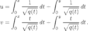
After Abel's premature death in 1829, Jacobi continued to develop algebraic function theory. In 1832, he realized that for algebraic integrals of higher genus, the limits of integration in the p integrals to which a sum was reduced could not be determined, since there were p integrals and only one equation connecting them to the variable in terms of which they were to be expressed. He therefore had the idea of adjoining extra equations in order to determine these limits. For example, if q(x) is of degree 5, he posed the problem of solving for x and y in terms of u and in the equations

This problem became known as the Jacobi inversion problem. Solving it took a quarter of a century and led to progress in both complex analysis and algebra.

41.2.3 Theta Functions

Jacobi himself gave this solution a start in connection with elliptic integrals. Although a nonconstant function that is analytic in the whole plane cannot be doubly periodic (because its absolute value cannot attain a maximum), a quotient of such functions can be, and Jacobi found the ideal numerators and denominators to use for expressing the doubly periodic elliptic functions as quotients: theta functions. The secret of solving the Jacobi inversion problem was to use theta functions in more than one complex variable, but working out the proper definition of those functions and the mechanics of applying them to the problem required the genius of Riemann and Weierstrass. These two giants of nineteenth-century mathematics solved the problem independently and simultaneously in 1856, but considerable preparatory work had been done in the meantime by other mathematicians. The importance of algebraic functions as the basic core of analytic function theory cannot be overemphasized. Klein (1926, p. 280) goes so far as to say that Weierstrass' purpose in life was

to conquer the inversion problem, even for hyperelliptic integrals of arbitrarily high order, as Jacobi had foresightedly posed it, perhaps even the problem for general abelian integrals, using rigorous, methodical work with power series (including series in several variables). It was in this way that the topic called the Weierstrass theory of analytic functions arose as a by-product.

41.2.4 Cauchy

Cauchy's name is associated most especially with one particular approach to the study of analytic functions of a complex variable, that based on complex integration. A complex variable is really two variables, as Cauchy was saying even as late as 1821. But a function is to be given by the same symbols, whether they denote real or complex numbers. When we integrate and differentiate a given function, which variable should we use? Cauchy discovered the answer, as early as 1814, when he first discussed such questions in print. The value of the function is a complex number that can also be represented in terms of two real numbers u and , as u + iv. If the derivative is to be independent of the real variable on which it is taken, these must satisfy the equations we now call the Cauchy–Riemann equations:

In that case, as Cauchy saw, if we are integrating u + iv in a purely formal way, separating real and imaginary parts, over a path from the lower left corner of a rectangle (x₀, y₀) to its upper right corner (x₁, y₁), the same result is obtained whether the integration proceeds first vertically, then horizontally or first horizontally, then vertically. As Gauss had noted as early as 1811, Cauchy observed that the function 1/(x + iy) did not have this property if the rectangle contained the point (0, 0). The difference between the two integrals in this case was 2πi, which Cauchy called the residue. Over the period from 1825 to 1840, Cauchy developed from this theorem what is now known as the Cauchy integral theorem, the Cauchy integral formula, Taylor's theorem, and the calculus of residues. The Cauchy integral theorem states that if γ is a closed curve inside a simply connected region⁶ in which f(z) has a derivative then

If the real and imaginary parts of this integral are written out and compared with the Cauchy–Riemann equations, this formula becomes a simple consequence of what is known as Green's theorem (the two-variable version of the divergence theorem), published in 1828 by George Green (1793–1841) and simultaneously in Russia by Mikhail Vasilevich Ostrogradskii (1801–1862). When combined with the fact that the integral of 1/z over a curve that winds once around 0 is 2πi, this theorem immediately yields as a consequence the Cauchy integral formula

When generalized, this formula becomes the residue theorem. Also from it, one can obtain estimates for the size of the derivatives. Finally, by expanding the denominator as a geometric series in powers of z − z₁, where z₁ lies inside the curve γ, one can obtain the Taylor series expansion of f(z). These theorems form the essential core of modern first courses in complex analysis. This work was supplemented by a paper of Pierre Laurent (1813–1854), submitted to the Paris Academy in 1843, in which power series expansions about isolated singularities (Laurent series) were studied.

Cauchy was aware of the difficulties that arise in the case of multivalued functions and introduced the idea of a barricade (ligne d'arrêt) to prevent a function from assuming more than one value at a given point. As mentioned in Section 38.3 of Chapter 38, his student Puiseux studied the behavior of algebraic functions in the neighborhood of what we now call branch points, which are points where the distinct values of a multi-valued function coalesce two or more at a time.

41.2.5 Riemann

The work of Puiseux on algebraic functions of a complex variable was to be subsumed in two major papers of Riemann. The first of these, his doctoral dissertation, contained the concept now known as a Riemann surface. It was aimed especially at simplifying the study of an algebraic function satisfying a polynomial equation . In a sense, the Riemann surface revealed that all the significant information about the function was contained precisely in its singularities—the way it branched at its branch points. Information about the surface was contained in its genus, defined as half the total number of branch points, counted according to order, less the number of sheets in the surface, plus 1.⁷ The Riemann surface of , for example, has two branch points (0 and ∞), each of order 1, and two sheets, resulting in genus 0.

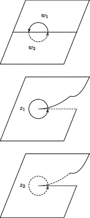
The smooth transition from z₁ to z₂ is shown in Fig. 41.3.⁸ The two z-planes are cut along the positive real axis or any other ray emanating from the “branch point” 0. Then the lower side of each cut is glued to the upper side of the other. (This will be easiest to visualize if you imagine the z₂-plane picked up and turned over so that the dotted edge of the z₂-plane lies on the dotted edge of the z₁ plane.) The result is the Riemann surface of the function . It consists of two “sheets” (copies of the complex plane) glued together as just stated. You can easily make a model of this surface with two sheets of paper, a pair of scissors, and cellophane tape. On such a model you can move your finger smoothly and continuously over the entire Riemann surface, without any jumps when it moves from the z₁ sheet to the z₂ sheet. In particular, if you describe a small circle about the branch point 0 at the end of the cut, you will see that it crosses over to the back of the paper when it moves across the dotted edges that have been glued together, makes a whole circle on the back, then crosses over again to the front when it moves across the solid line.

Figure 41.3 The Riemann surface of . The solid z₁ circle corresponds to the solid semicircle, and the dashed z₂ circle to the dashed semicircle.

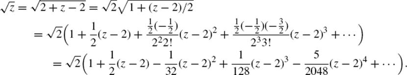
At every point on the Riemann surface except the branch point z = 0, the mapping is analytic; that is, it has a power-series representation. For example, near the point z₁ = 2, we can express as a series of powers of z − 2 using the binomial theorem:

Riemann's geometric approach to the subject brought out the duality between surfaces and mappings of them, encapsulated in a formula known as the Riemann–Roch theorem (after Gustav Roch, 1839–1866). This formula connects the dimension of the space of functions on a Riemann surface having prescribed zeros and poles (places where it becomes infinite) with the genus of the surface.

In 1856 Riemann used his theory to give a very elegant solution of the Jacobi inversion problem. Since an analytic function must be constant if it has no poles on a Riemann surface, it was possible to use the periods of the integrals that occur in the problem to determine the function up to a constant multiple and then to find quotients of theta functions having the same periods, thereby solving the problem.

41.2.6 Weierstrass

Of the three founders of analytic function theory, Weierstrass was the most methodical. He had found his own solution to the Jacobi inversion problem and submitted it simultaneously with Riemann. When he saw Riemann's work, he withdrew his own paper and spent many years working out in detail how the two approaches related to each other. Where Riemann had allowed his geometric intuition to build castles in the air, so to speak, Weierstrass was determined to anchor his ideas in a firm algebraic foundation. Instead of picturing kinematically a point wandering from one sheet of a Riemann surface to another, Weierstrass preferred a static object that he called a Gebilde(structure). His Gebilde was based on the set of pairs of complex numbers satisfying a polynomial equation , where was an irreducible polynomial in the two variables. These pairs were supplemented by certain ideal points of the form (z, ∞), , or (∞, ∞) when one or both of or z tended to infinity as the other approached a finite or infinite value. Around all but a finite set of points, it was possible to expand in an ordinary Taylor series in nonnegative integer powers of z − z₀. For each of the exceptional points, there would be one or more expansions in fractional or negative powers of z − z₀, as Puiseux and Laurent had found. These power series were Weierstrass' basic tool in analytic function theory.

41.3 Comparison of the Three Approaches

Cauchy's approach seems to subsume the work of both Riemann and Weierstrass. Riemann, to be sure, had a more elegant way of overcoming the difficulty presented by multivalued functions, but Cauchy and Puiseux between them came very close to doing something logically equivalent. Weierstrass began with the power series and considered only functions that have a power-series development. That requirement appears to eliminate a large number of functions from consideration at the very outset, whereas Cauchy assumed only that the function is continuously differentiable and only later showed that in fact it must have a power-series development.⁹

On the other hand, when this theory is applied to study a particular function, the apparently greater generality of Cauchy's approach seems less obvious. Before you can prove anything about the function using Cauchy's theorems, you must verify that the function is differentiable. In order to do that, you have to know the definition of the function. How is that definition to be communicated, if not through some formula like a power series or other well-known function whose analyticity is known? Weierstrass saw this point clearly; in 1884 he said, “No matter how you twist and turn, you cannot avoid using some sort of analytic expressions such as power series” (quoted by Siegmund-Schultze, 1988, p. 253).

Problems and Questions

Mathematical Problems

41.1. The formula cos θ = 4 cos ³(θ/3) − 3 cos (θ/3), can be rewritten as the equation p(cos θ/3, cos θ) = 0, where p(x, y) = 4x³ − 3x − y. Observe that cos (θ + 2mπ) = cos θ for all integers m, so that

for all integers m. That makes it very easy to construct the roots of the equation p(x, cos θ) = 0. They must be cos ((θ + 2mπ)/3) for m = 0, 1, 2. What is the analogous equation for dividing a circular arc into five equal pieces?

41.2. Suppose (as is the case for elliptic functions) that f(x) is doubly periodic, that is, f(x + mω₁ + nω₂) = f(x) for all m and n. Suppose also that there is a polynomial p(x) of degree n² such that p(f(θ/n)) = f(θ) for all θ. Finally, suppose you know a number say ϕ, such that f(ϕ) = C. Show that the roots of the equation p(x) = C must be x_m,n = f(ϕ/n + (k/n)ω₁ + (l/n)ω₂), where k and l range independently from 0 to n − 1.

41.3. Use L’Hospital's rule to verify that

for any function f(x) such that f ” (x) is continuous. Then suppose that f(x) = ∑ a_nxⁿ and g(x) = ∑ b_nxⁿ are two analytic functions on the interval −1 < x < 1 such that f(x) = g(x) for some interval −ε < x < ε for some positive number ε, no matter how small. Prove that f(0) = g(0), f′ (0) = g′ (0), and f ” (0) = g ” (0). (Similarly, it can be shown by using higher-order difference quotients of the function f to get its derivatives at 0 that f⁽ⁿ⁾(0) = g⁽ⁿ⁾(0) for all n. It then follows that a_n = f⁽ⁿ⁾(0)/n ! = g⁽ⁿ⁾(0)/n ! = b_n, and therefore that f(x) = g(x) everywhere. Thus, two analytic functions that coincide at all points in some interval around 0 must coincide everywhere.)

Historical Questions

41.4. What mathematical problems forced mathematicians to take complex numbers seriously instead of rejecting them as unusable?

41.5. What role did algebraic integrals play in the development of modern complex analysis?

41.6. What differences exist among the approaches of Cauchy, Riemann, and Weierstrass to the theory of analytic functions of a complex variable?

Questions for Reflection

41.7. We noted at the beginning of this chapter that convergent power series can represent only the ultra-smooth functions we call analytic, while convergent trigonometric series can represent functions that have very arbitrary breaks and kinks in their graphs. Considering that every complex number z has a polar representation z = r(cos θ + i sin θ), and zⁿ = rⁿ(cos (nθ) + i sin (nθ)), how do you account for this difference?

41.8. What value is there in starting from Cauchy's assumption that a function has a complex derivative at every point of a domain and then using the Cauchy integral to prove that it must then have a convergent power series expansion about each point? Weierstrass saw none, and preferred merely to start with the convergent power series as the definition of the function. Of course, it is easy to show that a convergent power series has a complex derivative at each point, so that the two definitions are equivalent. Is there an aesthetic or psychological reason for preferring one to the other?

41.9. Lagrange championed the use of analytic functions in physics because of the property that all the derivatives of an analytic function at a point can be computed (using higher-order differences) from the values of the function in an arbitrarily small neighborhood of the point. If the independent variable is time, this implies that the values the function over any time interval, no matter how short, determine its value at all subsequent times. In short, analytic functions are deterministic. How does this property mesh with the assumptions of classical physics? How would today's physicists look at it?

Notes

1. Hille (1959, p. 18) noted that the representation of complex numbers on the plane is called le diagramme d'Argand in France and credited the Norwegians with “becoming modesty” for not claiming det Wesselske planet.

2. The Czech scholar Bernard Bolzano (1781–1848) showed how to approach the idea of continuity analytically in an 1817 paper. His work anticipated Dedekind's arithmetization of real numbers, which will be discussed in the next chapter.

3. The simplest lemniscate, first described by James Bernoulli in 1694, is the set of points the product of whose distances from the points (+ a, 0) and (− a, 0) is a². It looks like a figure eight and has equation (x² + y²)² = 2a²(x² − y²).

4. Or, more generally, a Fermat prime number of parts.

5. To avoid complications, we are not discussing Legendre's three kinds of elliptic integrals. For those who know what they are, the results we state here should be assumed to apply only to integrals of first kind.

6. See Chapter 38 for the definition of a simply connected region.

7. Klein (1926, p. 258) ascribes this definition to Alfred Clebsch (1833–1872).

8. This figure is taken from the author's Classical Algebra (Wiley, 2008).

9. Cauchy assumed that the derivative was continuous. It was later shown by Edouard Goursat (1858–1936) in 1900 that differentiability implies continuous differentiability on open subsets of the plane.