Mathematics for the liberal arts (2013)

Part I. MATHEMATICS IN HISTORY

Chapter 3. MODERN MATHEMATICS

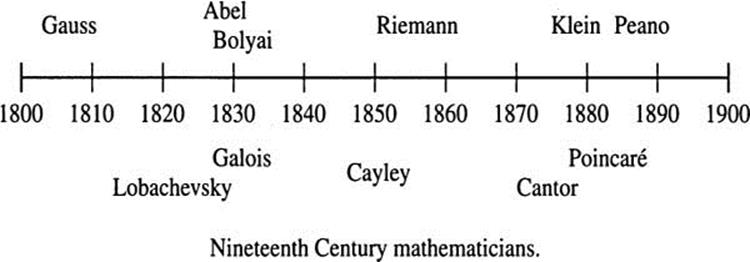
3.3 The 19th Century: Expansion

Introduction

The most important development of the 19th century was the continuation, indeed the acceleration, of the Industrial Revolution. Much of what we are today, we became in the 19th century.

In Europe, the early years of the century were dominated by the Napoleonic wars, which ended in 1815 with the defeat of France by a coalition of European powers. Great Britain emerged from these wars as the dominant power, a position it occupied through most of the century. This dominance was due to it being home to the Industrial Revolution. One estimate has the United Kingdom possessing about 20% of the world’s manufacturing production in 1860. (It had about 2% of the world’s population.) In 1900 London was the largest city in the world, with about 6.5 million people.

This was a century of empire. The biggest was of course the English empire, especially with its holdings in South Asia, crowned by India. But it also ruled over Canada, Australia, New Zealand and, later in the century, large parts of Africa. The other great European empire was the Russian, which ruled from Poland in the West to Alaska in the East. (The Russian Alaskan holdings were sold to the United States in 1867. There were also early Russian settlements in Hawaii and California.)

In Asia, this was a bad century for China. Its weakness was demonstrated by its defeat in the Opium Wars (1839–42 and 1856–60). China had tried to cut off the illegal importation of opium, controlled by the British, but were defeated and required to make major trade concessions. Partly as a consequence, China was convulsed by the Taiping Rebellion (1850–64), in which about 20 million people died.

Following the forcible opening of Japan to Western trade by the American Commodore Matthew Perry in 1853, Japan rapidly adopted Western technology and industry. By century’s end, it had become a major imperial power, defeating China in a war in 1895 and Russia ten years later.

Not all empires prospered at this time. The Spanish and Portuguese empires in America collapsed in the early years of the century. Between 1810 and 1822, independence from Spain and Portugal was obtained by nearly the entire South American continent, as well as Mexico.

The second half of the 19th century saw the rise of two new powers: Germany and the United States. Germany was united from a number of smaller states by the Prussian Otto von Bismarck. By the time of the Franco-Prussian War (1870–71), Germany was the continent’s most powerful country. Also at this time, America was emerging from its civil war, and rapidly industrializing.

Overshadowing these changes was the Industrial Revolution. This century saw the spread of the previous century’s innovations. To these were added diverse new technologies. The telegraph, the Internet of its day, for the first time allowed people many miles apart to communicate almost instantaneously. The railroad revolutionized transportation. The electric motor was invented, followed by the electric grid and the electric light. The telephone changed the world of communication. World trade expanded. The Suez Canal opened in 1869. Refrigeration was invented, allowing, for example, meat to be shipped from Argentina to Europe. The population of Europe roughly doubled in this century, as it had in the previous one.

These changes in technology were accompanied by equally important cultural and political changes. People started moving from farms into cities. Some parts of the world, including Britain and America, saw a gradual expansion of democracy. Slavery was abolished in the United States after the Civil War. Russia emancipated its serfs in 1861.

The nineteenth was a great century for “isms.” In addition to imperialism and colonialism, Europe saw a surge in nationalism, including the unification of both Germany and Italy. Socialism, communism, and anarchism all arose in response to the problems created by the new industrialization, including appalling urban squalor (see Dickens).

Supported by the new wealth, the arts flourished in this century. A (somewhat arbitrary) hall of fame would include Johann Wolfgang von Goethe and Jane Austen, Vincent van Gogh and Auguste Rodin, Ludwig van Beethoven and Antonin Dvorak and Peter Ilyich Tchaikovsky, Richard Wagner and Giuseppe Verdi and Georges Bizet, Charles Dickens and Fyodor Dostoyevsky and Mark Twain.

The word “scientist” originated in this century, and science produced many advances. Physicists achieved a remarkable unification of electric and magnetic phenomena. Michael Faraday (1791–1867) performed experiments that elucidated the nature of electromagnetism, and invented the electric motor. James Clerk Maxwell (1831–1879) discovered that light was an electromagnetic wave, and reduced all of electricity and magnetism to four equations.

Also in physics, the study of heat and energy led to the development of thermodynamics and statistical mechanics. Some of the important contributors were Sadi Carnot (1796–1832), Rudolf Clausius (1822–1888), William Thomson, Lord Kelvin (1824–1907), Ludwig Eduard Boltzmann (1844–1906), and Josiah Willard Gibbs (1839–1903) (who worked in relative obscurity in America).

In chemistry, John Dalton (1766–1844) developed the modem theory of atoms. Dmitry Ivanovich Mendeleev (1834–1907) constructed his periodic table of elements, and used it to predict three new elements–germanium, gallium, and scandium–which were later discovered.

Biology saw the publication in 1859 of On the Origin of Species by Charles Darwin (1809–1882), which provided a theoretical foundation for biological evolution. This theory was independently proposed by Alfred Russel Wallace (1823–1913), an outgrowth of his herculean efforts as a professional collector of biological specimens from around the world. (In his eight years exploring the East Indies, he collected, cataloged, and returned to England 125,660 plant and animal specimens, including 83,000 beetles.) The germ theory of disease, with its profound implications for public health, was developed by Louis Pasteur (1822–1895), Joseph Lister (1827–1912), and Robert Koch (1843–1910).

Mathematics thrived in the 19th century. There was progress on old problems, such as which figures can be constructed using compass and straightedge, and solving fifth degree polynomials. The foundations of mathematics were elucidated, with formal definitions of integers and real numbers. The analysis of complex numbers continued, with major applications to physics and to other areas of mathematics. Perhaps most impressive were the new topics: Fourier analysis, non-Euclidean geometry, vectors and matrices, logic and set theory, and abstract group theory.

Complex Variables

In the previous section, we mentioned the advent of complex numbers. AugustinLouis Cauchy (1789–1857) and Georg Friedrich Bernhard Riemann (1826–1866) further developed this branch of mathematics by studying complex functions, which are functions from the complex plane to the complex plane. These are more difficult to picture than real functions, because both the domain and the range are 2-dimensional. However, complex functions have elegant properties that make them, in some respects, better behaved than real functions. For example, the real function f(x) = x^5/3 has a derivative easily obtained by the power rule: f′(x) = (5/3)x^2/3. However, using the power rule again, the second derivative, f″(x) = (10/9)x^–1/3, is not defined at 0. By contrast, when a complex function has a derivative, all higher order derivatives exist. A differentiable complex function is called an analytic function. Analytic functions can be expanded in terms of power series (infinite polynomials). For instance, the exponential function f(z) = e^z has the power series expansion

While the real exponential function is always nonnegative, the complex exponential function takes all complex values except 0.

Complex variables have proven to be a powerful tool in many branches of mathematics, including number theory.

Number Theory

In 1796 Gauss showed that a regular polygon with 17 sides is constructible using only a straightedge and compass. This result, first appearing in Gauss’s Disquisitiones Arithmeticae (1801), extends Euclid’s Elements, where constructions of an equilateral triangle and a regular pentagon are given. Gauss went on to show that a regular polygon with n sides is constructible if n is either a power of 2 or n = 2^mp₁p₂ … p_r, where m ≥ 0 and p₁,P₂,…, p_r are distinct primes of the form 2^2k + 1, for k ≥ 0. Some admissible values of n are 3, 5, 20 = 2² · 5, and 85 = 5 · 17, while some inadmissible values are 7, 13, and 25 = 5². Primes of the required form are called Fermat primes. Indeed, 2^2k+ 1 is a prime for k = 0,1, 2, 3, and 4, but for no known higher values of k.

Carl Friedrich Gauss (1777–1855)

Carl Friedrich Gauss was bom into a poor family in Brunswick, Germany. He showed strong mathematical ability at an early age. One story has it that at age ten he surprised his teacher by adding all the numbers from 1 to 100 instantly. He did this by pairing 1 and 99, 2 and 98, 3 and 97, etc. The forty-nine pairs that sum to 100 total 4900. Together with 50 and 100, this totals 5050. Thus, Gauss found the formula

which we encountered in Chapter 1.

Gauss’ teachers recognized his genius, and, beginning in 1791, the Duke of Brunswick financed his education. Gauss studied at the University of Göttingen from 1795 to 1798, then obtained his doctorate at the University of Helmstedt. He joined the University of Göttingen as professor of astronomy in 1807, and remained there for the rest of his life.

Like Euler, Gauss was a mathematical titan who reinvigorated traditional areas of mathematics, inaugurated new fields, and made many discoveries that now bear his name. His research transformed nearly all branches of mathematics, including number theory, geometry, algebra, analysis, and probability, as well as physics.

Gauss became quite famous in 1801 for his rediscovery of the asteroid Ceres, which had been discovered earlier, but lost because its orbit was not known. This rediscovery was made possible by Gauss’ development–at age eighteen–of a method to handle experimental errors, the method of least squares.

Also in 1801 Gauss published Disquisitiones Arithmeticae (Research in Number Theory). This monograph encompasses discoveries by past mathematicians and Gauss’s new contributions. In the preface, Gauss acknowledges four predecessors: Euler, Fermat, Lagrange, and Legendre. An important element of the work is Gauss’s new congruence notation. (See Chapter 5.)

Gauss worked extensively in geometry, studying alternative geometries to Euclidean geometry (non-Euclidean geometries). He also laid the foundations for differential geometry, which uses calculus to study geometrical curves and surfaces.

Gauss is renowned in physics as well, for many discoveries. In 1833 he and Wilhelm Weber invented an early electric telegraph, able to communicate over a distance of 1200 meters.

Gauss gave four proofs of the Fundamental Theorem of Algebra, probably because he considered the theorem so important. He gave the final proof when he was in his 70s.

The most important development in number theory in the 19th century was crossfertilization with other branches of mathematics, such as complex variables and group theory. Recall that Lagrange had proved that every positive integer is the sum of four squares. In 1834 Carl Gustav Jakob Jacobi (1804–1851) extended Lagrange’s theorem by finding a formula for the number of ways that an integer n can be written as the sum of four squares. The formula depends on whether n is odd or even. If n is odd, then the number of ways that n can be written as a sum of four squares is 8 times the sum of the positive divisors of n. If n is even, it is 24 times the sum of the odd positive divisors of n. We posed the question, how many ways can you write 10 as a sum of four squares (where the order of the terms and the sign of the numbers being squared is important)? According to Jacobi’s formula, the number of ways is

The proof of Jacobi’s theorem uses the theory of complex variables.

The crowning achievement in number theory in the 19th century was the proof of the Prime Number Theorem in 1896, by Jacques Hadamard ( 1865–1963) and Charles Jean de la Vallée-Poussin (1866–1962). The theorem, described in the previous section, was conjectured by Gauss and Legendre. Its proof uses functions of complex variables.

The Quintic

In Chapter 2 we discussed the fact that cubic and quartic equations are solvable using the four arithmetic operations (addition, subtraction, multiplication, and division) and radicals (square roots, cube roots, etc.). After the discovery of these solutions, mathematicians sought to solve the quintic equation,

Lagrange had set the stage for understanding solutions of equations by introducing one of the most important ideas: permutations of roots of a polynomial. A permutation is a rearrangement. For example, shuffling a deck of cards is a permutation of the 52 cards. Lagrange’s concept of permutations of polynomial roots led to breakthroughs in polynomial theory by Abel and Galois, and to the development of group theory, with implications throughout mathematics.

Niels Abel (1802–1829) proved that there are quintics that cannot be solved by radicals, showing in particular that x⁵ – 10x + 2 is not solvable. Évariste Galois (1811–1832) later provided a more general theory for which quintics are solvable. He had the key insight that a polynomial can be solved in radicals if and only if its associated Galois group (a set of permutations of its roots) is “solvable.” (A solvable group can be built up from commutative groups–groups in which xy = yx for all elements x and y.) The Galois group of Abel’s example consists of all permutations of the five roots. This group is unsolvable.

Niels Henrik Abel (1802–1829)

Niels Henrik Abel was bom on the island of Finϕy, in southwestern Norway, but spent most of his life in southeastern Norway. The family was poor, and the situation grew worse when Abel’s father, a Lutheran minister, died in 1820. Abel’s mathematics teacher raised funds for his education, however, and he was able to attend the University of Christiania in Oslo. He never was able to find a university position, and died of tuberculosis at age 26.

Abel is perhaps most famous for proving the impossibility of solving the quintic by radicals (mentioned above), but contributed to many areas of mathematics. His contributions are memorialized in terms including abelian groups, abelian functions and abelian integrals. In 2002 the Abel Prize, a prestigious mathematical award, was created in his honor.

Évariste Galois (1811-1832)

Évariste Galois was bom in Bourg-la-Reine, a town near Paris. His education was spotty: he twice failed the entrance examination for the École Polytechnique, instead attending the École Normale, a school for training teachers. Galois then became involved in the chaotic politics of the time, and was expelled from that school.

Galois submitted several papers on polynomial equations to the Academy of Sciences. A couple of times they lost his manuscripts. Augustin-Louis Cauchy did review two of his papers, but did not publish them.

Galois died at age 20, of injuries sustained in a duel. He stayed up the night before, writing a letter to a friend; including several manuscripts with some annotations. The letter concluded: “Ask Jacobi or Gauss publicly to give their opinion, not as to the truth, but as to the importance of these theorems. Later there will be, I hope, some people who will find it to their advantage to decipher all this mess.” His manuscripts were finally published in 1846, but not fully appreciated for decades after that.

In his short, tragic life, Galois had monumental mathematical insights. He was the first to use the word group (“groupe,” in French) to refer to a collection of permutations. The concept of a group has since become enormously important in mathematics. Galois was also the first to describe and investigate finite fields (see Chapter 5). The great Hermann Weyl (1885–1955) wrote of Galois’ last testament: “This letter, if judged by the novelty and profundity of ideas it contains, is perhaps the most substantial piece of writing in the whole literature of mankind.”

The Abstract Concept of a Group

The groups studied by Galois and Abel were groups of permutations of roots of polynomials. Cauchy studied more general permutation groups. Arthur Cayley (1821–1895) gave the first abstract definition of a group in 1854: A group is a set together with an operation on pairs of elements of the set. Suppose that we indicate the operation on x and y by xy. (The operation might not be commutative, that is, xy doesn’t necessarily equal yx.) The operation must be associative: (xy)z = x(yz), for all elements x, y, and z. There must be an identity element, e, such that xe = ex = x, for all elements x. Finally, each element x must have an inverse, x^–1, such that xx^–l = x^–lx = e. An example of a group is the set of positive real numbers, with the operation multiplication. The identity element is 1. Each positive real number x has a multiplicative inverse 1/x.

Arthur Cayley (1821–895)

Arthur Cayley was bom in England, but spent most of his first seven years in Russia, where his merchant father moved the family, before returning to England. He showed early talent in mathematics, and entered the University of Cambridge at the age of 17. He stayed some years at Cambridge as student and fellow, but left in 1846 to study law. He practiced law for 14 years, while producing over 300 mathematics papers in his spare time.

At the age of 42, Cayley gave up his lucrative legal career to become a professor of mathematics at Cambridge. He stayed at Cambridge the rest of his life, continuing to produce research at a prodigious rate. He was also an early supporter of university education for women, and served in the 1880s as chairman of the council of Newnham College, one of the two women’s colleges at Cambridge.

Cayley wrote over 900 mathematical papers in the areas of algebra, including linear algebra and abstract algebra, geometry, differential equations, and combinatorics. His conception of matrix algebra would prove to be important in quantum mechanics in the next century.

Non-Euclidean Geometry

Recall from Chapter 1 that Euclid’s Elements contains five postulates, the fifth of which is more complicated than the other four. The fifth postulate is equivalent to the following statement about the existence of parallel lines:

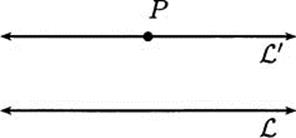
Given a line and a point P not on , there exists a unique line passing through P which does not intersect

We say that is parallel to (Figure 3.12).

Over the next two thousand years, mathematicians attempted to prove Euclid’s fifth postulate from the other four. Some thought they had succeeded, but there was always a mistake in the reasoning. Finally, it became clear that the fifth postulate cannot be proved from the first four. One can assume that the postulate is false and derive consistent geometry that is quite different from Euclidean geometry. A geometry in which Euclid’s fifth postulate does not hold is called a non-Euclidean geometry.

Figure 3.12 A parallel line given by Euclid’s fifth postulate.

If the fifth postulate is false, there are two possibilities: (1) there are no lines parallel to a given line and passing through a given point; or (2) there is more than one such parallel line. The first case is called elliptic geometry; the second case is called hyperbolic geometry. (These terms were introduced by Felix Klein.)

In the early 1800s, the Hungarian mathematician Janos Bolyai (1802–1860) and the Russian mathematician Nikolai Ivanovich Lobachevsky (1792–1856) formulated versions of hyperbolic geometry. Gauss had discovered hyperbolic geometry earlier but didn’t publish his findings. Later, Bernhard Riemann (1826–1866) formulated elliptic geometry.

Nikolay Ivanovich Lobachevsky (1792–1856)

Nikolay Ivanovich Lobachevsky’s father died when he was young, and his mother moved to Kazan, a Russian city about 700 kilometers east of Moscow, just west of Siberia. Lobachevsky studied at the Kazan State University, where most of his teachers were German. He later joined the faculty there, and was promoted to full professor in 1822. He served as rector of Kazan University from 1827 to 1846, when he retired. The university prospered in his time as rector, and he worked to improve education throughout the entire Kazan district.

Lobachevsky’s first paper on non-Euclidean geometry was written in 1823, but not published until much later. His first work on the subject to make it to print appeared in an obscure Kazan journal in 1829. A later text of his was praised by Gauss in 1842, but not everyone appreciated the new geometry. Lobachevsky’s work did not receive full recognition until after his death, with the work of Riemann and Klein.

Lobachevsky worked in other areas of mathematics as well. There is a method still used to approximate solutions of algebraic equations, called the Lobachevsky–Gräffe or Dandelin–Gräffe method, discovered independently by Lobachevsky, Germinal Pierre Dandelin (1794–1847), and Karl Heinrich Gräffe (1799–1873).

János Bolyai (1802–1860)

János Bolyai was the son of a Hungarian mathematician, Farkas Bolyai. János was a prodigy, but his family could not afford to send him to a first-rate university. Instead, he studied at the Royal Engineering College in Vienna, completing the seven year course in four years. He then served in the Austro-Hungarian Imperial Army engineering corps from 1822 to 1833. He was a renowned swordsman, as well as an accomplished violinist, and spoke at least nine languages.

Bolyai’s father encouraged him in his mathematics, but tried to dissuade him from studying Euclid’s fifth postulate, having studied it himself to no avail. Janos ignored the warning, and instead produced a consistent geometry that did not obey the fifth postulate. In 1832 this work appeared as an “Appendix Explaining the Absolutely True Science of Space” in his father’s textbook An Attempt to Introduce Studious Youth to the Elements of Pure Mathematics.

Carl Friedrich Gauss had discovered a non-Euclidean geometry earlier, but had not published his work. When he read Bolyai’s appendix, he wrote to a friend, “I regard this young geometer Bolyai as a genius of the first order.” Gauss’s letter to his friend Farkas Bolyai on his son’s work was less than tactful, however: “To praise it would amount to praising myself. For the entire content of the work…coincides almost exactly with my own meditations which have occupied my mind for the past thirty or thirty-five years.” This response was a blow to Janos. A further blow was his discovery, in 1848, that Lobachevsky had published a similar geometry in 1829. As was the case with Lobachevsky, Bolyai’s work was not fully appreciated until after his death.

In Euclidean geometry, the sum of the angles of a triangle is 180°. In elliptic geometry, the sum of the angles is greater than 180°, while in hyperbolic geometry, the sum is less than 180°. In hyperbolic geometry, all similar triangles have the same area.

Besides providing new mathematical worlds to explore, non-Euclidean geometries point to a more axiomatic—and less intuitive—trend in mathematics. It had been taken for granted that Euclidean geometry was the geometry, but now we realize that this geometry is only a logical extension of the axioms we assume, and these axioms do not necessarily represent logical or physical truth. In fact, it is not known what geometry provides the best model of the physical universe. More and more, mathematicians would emphasize the logical foundations of the various branches of their discipline. This would ultimately lead to a réévaluation of mathematical logic itself in the 20th century.

Bernhard Riemann (1826–1866)

Georg Friedrich Bernhard Riemann was bom in the village of Breselenz, in northern Germany, the son of a Lutheran pastor. The family was relatively poor, but found enough money to send Bernhard to the University of Gottingen, to study theology. He soon switched to mathematics, moved to the University of Berlin for two years, then returned to Gottingen, where he completed his dissertation under Gauss’s supervision. He spent most of the rest of his career at Gottingen, eventually being appointed to the mathematics professorship in 1859.

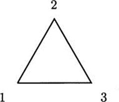
Figure 3.13 An equilateral triangle has six symmetries.

Riemann contributed to many areas of mathematics, and to physics. He is best known for his work in geometry. Riemannian geometry, as it is now called, is the mathematical foundation of Einstein’s general relativity. Riemann’s work in geometry also inspired the work of another mathematician, Charles Lutwidge Dodgson (aka Lewis Carroll). The looking glass connecting England to Wonderland in Carroll’s Through the Looking-Glass was an example of a Riemann cut, the original of what is now called a wormhole.

Riemann published only one paper in number theory, eight pages long. In it, he applied new ideas in complex analysis, and produced probably the leading unsolved problem in mathematics today, the Riemann Conjecture. The solution of the Riemann Conjecture would yield important results on the distribution of prime numbers, and will eventually win someone one million dollars.

Riemann also did important work on the foundations of calculus. See, for example, Sections 4.14 and 4.15.

In 1862 Riemann fell ill with tuberculosis. In the next few years, he made several trips to Italy to treat the disease, but eventually succumbed to it. He died in Selasca, Italy, at the age of 39.

Groups and Geometry

Recall that a group is a set with an operation satisfying certain properties. Groups can describe the symmetries of an object.

Here is a small example. Consider the equilateral triangle in Figure 3.13, whose vertices are numbered 1, 2, and 3.

An equilateral triangle can be rotated or flipped over and occupy the same space. There are six symmetries, including all rotations and flipping over the triangle. The group consists of these six symmetries, where the operation is performing one symmetry after another (this is called composition). The group contains a smaller group of three symmetries, namely, the three rotations. (One of the rotations is the identity element, which leaves the triangle unmoved.) The smaller group is a subgroup of the larger group.

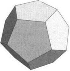
The five Platonic solids (tetrahedron, cube, octahedron, dodecahedron, and icosahedron) have symmetry groups. Let’s consider the dodecahedron (Figure 3.14). It has twelve faces which are regular pentagons. The dodecahedron can be picked up and set down on any of its twelve faces. Then it can be rotated into any one of five positions. After these maneuvers, the dodecahedron occupies its original space. Since there are twelve choices for which face goes on the bottom, and five choices for the rotation, there are altogether 12 · 5 = 60 symmetries of the dodecahedron. This 60-element group is “simple,” meaning that it cannot be broken down into smaller symmetry groups.

Figure 3.14 The dodecahedron has 60 symmetries.

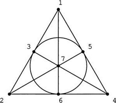
We will give another example of a symmetry group. Figure 3.15 shows a finite geometry with seven points and seven lines. The points are labeled 1, 2, 3, 4, 5, 6, 7. The lines are 123, 154, 264, 176, 374, 275, 356. Points are collinear if they lie on the same line. For example, 1, 4 and 5 are collinear, while 1, 4, and 7 are not collinear. In finite geometry, the only thing that matters is the relationship between points and lines. The points can be placed anywhere and the lines can be drawn curved or straight. Notice that the line 356 looks like a circle in our diagram. This finite geometry has one of the properties of Euclidean geometry: for every two points there is a unique line containing them. But every two lines intersect; there are no parallel lines, so this is a non-Euclidean geometry.

A symmetry of this finite geometry is a way of relabeling the points so that all the collinearity relationships are preserved. For instance, if we simply switched labels 1 and 2, we would mess up the collinearity, since 1, 5, and 4 would no longer be collinear (for example). In a symmetry, lines have to stay lines. How many symmetries does the finite geometry have? We know that there are 7! possible permutations of the seven point labels, but as we have seen, not all permutations are symmetries. All seven points are interchangeable, since they are all on the same number of lines (three). We are therefore free to relabel point 1 as any of the seven points (including leaving it as 1). Say we label it 1′. Once this decision is made, we can relabel 2 with any label other than 1′. There are six choices. So far, we have been free to make 7 o 6 choices. Once we relabel 1 and 2, we are forced (by collinearity) to choose for 3 the label of the point collinear with the 1′ and 2′. However, now that we have relabeled 1, 2, and 3, we can relabel 4 with any label not already used (four choices). Once we relabel 4, collinearity forces all of the other labeling decisions. Altogether, there are 7 · 6 · 4 = 168 ways to relabel the finite geometry, and that is the number of symmetries. Since the symmetries form a group, this establishes a group of 168 elements (one element for each hour of the week!). Like the symmetry group of the dodecahedron, this group is simple.

Figure 3.15 A finite geometry with 168 symmetries.

Let’s bring the discussion back to Euclidean geometry. When we say that two figures are congruent in Euclidean geometry, we mean that there is a motion that brings one figure into the other. Such a motion must be “rigid” in that it preserves all lengths of line segments and angles. We call these motions isometries of the plane.

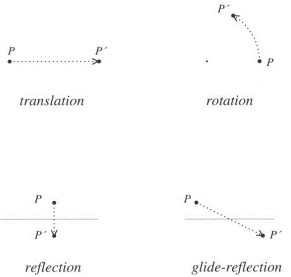
There are four types of isometries of the plane, as shown in Figure 3.16. The first two, translations and rotations, preserve orientation of the plane. If you translate or rotate a picture of a left-handed glove, it will stay left-handed. The other two isometries, reflections and glide-reflections, reverse orientation. They give a mirror image of a figure. A left-handed glove would be transformed into a right-handed glove. The collection of isometries, under composition, forms a group.

Felix Klein (1849–1925), while at the university at Erlangen, Germany, proposed his Erlangen Program (1872), in which he emphasized that geometry should be studied according to its symmetries. Thus, all the properties of Euclidean geometry are inherent in the group of isometries. Other geometries have different notions of equivalence and therefore different symmetry groups. The wider the definition of equivalence, the larger the corresponding symmetry group.

Figure 3.16 The four types of isometries of the plane.

Klein showed that the geometries known in his time–Euclidean, non-Euclidean, and projective–can all be viewed as instances of projective geometry. (Examples of projective geometry are perspective geometry, discussed in Chapter 2, and the finite geometry of Figure 3.15.) Projective geometry is therefore very general; there are more symmetries than in the special cases of Euclidean and non-Euclidean geometry; correspondingly, there are fewer “invariants,” properties retained under symmetry. For example, there are no angles in perspective geometry. (When you look at a square from a slant-wise perspective, its right angles become slanted.)

Felix Klein (1849–1925)

Christian Felix Klein was bom in Düsseldorf, Prussia (now in western Germany), the son of a government official. He studied physics and mathematics at the University of Bonn.

In 1872, at the age of 23, he was appointed professor at the University of Erlangen. It was on the occasion of this appointment that he set out his Erlangen Program. He subsequently worked at the Institute of Technology in Munich (1875–80), the University of Leipzig (1880–86), and finally at the University of G–ttingen (1886–1913).

Klein built Göttingen into one of the leading research centers of its day and, as editor, turned the Mathematische Annalen into one of the leading mathematical research journals. He supervised the dissertation of Grace Chisholm Young, who in 1895 was the first woman to earn a doctorate in Germany, in any field. Klein also worked to improve the teaching of mathematics in secondary schools.

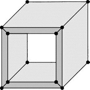
Figure 3.17 A polyhedron with a hole.

From Galois’ concept of a group of permutations of the roots of a polynomial, to the abstract definition of a group, to the use of groups in geometry, the rise of group theory has been a vital and increasingly important part of modem mathematics.

Topology

In Euclidean geometry, two figures are “the same” if they congruent. In Chapter 2 we saw that in perspective geometry figures need not be congruent to be considered “the same.” Any two quadrilaterals are “the same” in perspective geometry.

Topology is a type of geometry in which shapes can twist, bend, and stretch, but not break. Let us use the term equivalent for “the same.” In topology, two figures are equivalent if we can bend, stretch, and twist one figure to make it identical to the other.

An easy-to-understand example of topology is the equivalence between a doughnut with one hole and a coffee cup with a handle. The two shapes are equivalent because one can be deformed into the other (if they are malleable) by bending, stretching, and twisting. The common shape is called a torus. We will see a construction of a torus in the forthcoming discussion of graph theory.

Let’s take a look at the relevance of topology to a formula of Euler that we examined earlier. Euler’s formula states that V – E + F = 2, for a polyhedron with V vertices, E edges, and F faces. We stipulated that the polyhedron has no holes. Figure 3.17 shows a polyhedron with a hole. The shape is topologically equivalent to a torus.

For this polyhedron, V = 16, E = 32, and F = 16. Notice that Euler’s formula does not hold. However, Euler discovered a generalization of his formula, later further generalized by Henri Poincare, that relates V, E, and F to the number of holes, g, in the polyhedron:

If g = 0 (no holes), we are back to Euler’s original formula. For the polyhedron in Figure 3.17, we have g = 1 and V – E + F = 2 – 2·1 = 0.

A polyhedron with g holes is topologically equivalent to a smooth surface with g holes. We call g the genus of the surface. These kinds of surfaces are all orientable, meaning that if you put a clock face on the surface and move it around, it will always keep time in a clockwise fashion. Other surfaces are nonorientable. Whether orientable or nonorientable, surfaces are called (two-dimensional) manifolds. A manifold is a geometry that is locally like Euclidean space. A person who inhabited a small region of a manifold wouldn’t know the difference between it and the plane. Three-dimensional manifolds are more complicated, and they are still not fully understood.

Discoveries in topology may tell us something about the shape of the universe. It is not known what the true topology of the universe is.

Henri Poincaré (1854–1912)

Henri Poincaré was bom in Nancy, France, the son of a medical professor. The family was prominent; a cousin was President of France during World War I.

Poincaré obtained his doctorate from the École Polytechnique in 1879, studying differential equations. While working on his mathematics doctorate, he also got a degree in engineering. He taught at the University of Caen for two years, then joined the University of Paris, where he remained for the rest of his life.

In 1886 King Oscar II of Sweden offered a prize to anyone who could establish whether the solar system is stable, so that planets won’t fly off into space or crash into one another. Poincaré began his study of the problem by considering a simpler one, a system with three objects, the 3-body problem. (The 2-body problem had already been solved.) He found this to be difficult enough, but his proof that 3-body systems are stable won the prize. After the prize was awarded, and his paper printed, Poincaré discovered an error. He rewrote the paper and paid for it to be reprinted (costing him more than he had won), in the process proving that the solution of the 3-body problem cannot be written as a formula, and that the system is chaotic. Small changes in the initial positions of the bodies can lead to large differences later. This was the origin of chaos theory, which became an important area of mathematics in the second half of the 20th century.

Poincaré did other important work in physics and astronomy, including relativity theory, and in many areas of mathematics. But he is known best for his work in topology, and is often called the father of algebraic topology. He formulated what has become known as the Poincaré Conjecture, which concerns three-dimensional manifolds. This conjecture attracted the attention of some of the best mathematicians, leading to Fields Medals (the mathematical equivalent of Nobel Prize) in 1966, 1986, and 2006, when the conjecture was finally proved.

Mathematical Analysis

When calculus was unleashed upon the world in the 1600s, it was an instant success. Mathematicians and physicists realized that it provided a mathematical framework in which major problems could be expressed and solved. Calculus explained Kepler’s planetary laws. Calculus explained the tidal effects of the Moon. In our age, calculus has taken astronauts to the Moon and back to Earth.

However, the foundations of calculus were a little shaky from the start. Newton wrote his Philosophice Naturalis Principia Mathematica in the language of geometry. When he needed to justify a limit, he used complicated geometrical reasoning. Leibniz, on the other hand, offered a new mathematical object–the infinitesimal. The derivative (rate of change) of the function y with respect to the variable x is dy/dx, where the “differentials” dy and dxrepresent infinitesimal changes in y and x, respectively. In a later publication, Newton introduced the terms “fluent” for function and “fluxion” for derivative, an appeal to physical intuition that didn’t help to clear up matters.

The philosopher George Berkeley (1685–1753), not liking infinitesimals or fluxions, gave a biting critique of calculus in a book titled The Analyst (1734):

And what are these Fluxions? The Velocities of evanescent Increments? And what are these same evanescent Increments? They are neither finite Quantities nor Quantities infinitely small, nor yet nothing. May we not call them the ghosts of departed quantities?

Although calculus was practical and popular, some shoring up of its foundations was in order.

The two main operations of calculus are differentiation and integration. Both are defined in terms of limits. To give calculus a firm foundation, limits must be defined carefully. This was first done in 1817 by Bernard Bolzano (1781–1848). The “epsilon-delta” definition quantifies the relationships among the function, the independent variable, and the limit. For the record, the definition is that the limit of the function f(x), as x approaches a, is L, or in symbols,

if for every positive number ε, there exists a positive number δ, such that for all x satisfying 0 < |x – a| < δ, we have |f(x) – L| < ε. This is a precise way of saying that f(x) gets as close as we like to L when x is sufficiently close to a.

With the definition of limit, we define a function f to be continuous at a point a if This rigorously captures the commonplace idea of a continuous function being one that can be drawn without lifting one’s pen.

Having a rigorous definition of limit puts calculus on a sound basis, but it raises other issues. Once the definition is accepted, it is tested against various kinds of “pathological functions,” which are functions with strange properties. Mathematicians delighted in finding functions that are nowhere continuous, or continuous only at one point, or everywhere continuous and nowhere differentiable. Giuseppe Peano (1858–1932) found, in 1890, a one-dimensional curve that fills the entire plane. He was motivated by Georg Cantor’s theory of infinite sets, which establishes a one-to-one correspondence between the points on a line and the points in the plane, so that the two sets have the same cardinality (size).

Pathological functions have changed the landscape of mathematics. Any theory must account for them. An irony of pathological functions is that they are actually the “normal functions.” Most functions (in a precise mathematical sense) are pathological. The functions that we ordinarily encounter (polynomial, rational, trigonometric, exponential, logarithmic, etc.) are atypical.

Giuseppe Peano (1858–1932)

Giuseppe Peano was bom on a farm in northwestern Italy. He was educated in nearby Turin, and taught at the University of Turin from 1880 until the day he died.

Besides the space-filling curve mentioned above, he is best known for the Peano Axioms. These axioms provide a rigorous foundation for the positive integers, from which true statements about the positive integers (theorems) can be deduced. Peano also introduced several symbols of set theory that are commonly used today, e.g., union (∪), intersection (∩), “element of” (∈), and “subset of” (⊂).

Peano wrote textbooks for mathematicians at all levels, including for secondary school teachers, and was the creator and advocate of a universal language based on Latin, French, German and English.

Mathematical Logic

Much of the mathematical theory behind modem computers was invented in the 1800s. Charles Babbage (1791–1871) created a plan for what he called an “Analytical Engine,” a machine capable of arithmetic operations and memory. Although it hasn’t been built yet (a project to do so is now underway), its design envisioned all of the concepts necessary for modem computing. Ada Lovelace (1815–1852), often called the first computer programmer, wrote the first computer algorithm for this machine.

The mathematical underpinnings of computing were developed at the same time as a new understanding of logic was achieved, and these advances went hand-in- hand. One of the major mathematical contributions was propositional calculus. A proposition is a statement that is true or false. A calculus is a system of calculations. So, a propositional calculus is a way of calculating with statements.

Statements can be simple, such as “The cat is in the snow,” or fantastic. Lewis Carroll (1832–1898) offered many delightfully convoluted propositions in his Symbolic Logic (1897). Some examples:

“Animals, that do not kick, are always unexcitable.”

“No plum-pudding, that has not been boiled in a cloth, can be distinguished from soup.”

“A man, who has lost money and does not eat pork-chops for supper, had better take to cab-driving, unless he gets up at 5 a.m.”

The point is that no matter how ridiculous the statements, they may be deemed either true or false.

Statements can be combined with connectives to make new statements. The simplest connectives are ‘or’ and ‘and’. If p and q are statements, we write

for ‘or’ and ‘and’, respectively. By definition, p ∨ q is true when p or q is true; p∧q is true when both p and q are true. The operation ‘not’ specifies the negation of a statement. The notation ~ p represents ‘not’ p. Thus, ~ p is true when p is false.

A statement that is always true is called a tautology. An example is p∨ ~ p, because, for every statement p, either p or its negation is true. An example in words:

‘It is raining carrots or it is not raining carrots.”

George Boole (1815–1864), in his book Laws of Thought (1854), showed that combinations of statements can be manipulated algebraically. If p is a proposition, we introduce a variable P which equals 0 or 1 depending on whether p is true or false. If p is true, then P = 1. If p is false, then P = 0. The propositional calculus with these variables is called Boolean algebra. In Boolean algebra, the ‘or’ operation is usually written with a ‘+’ symbol, while the ‘and’ operation is written with a ‘·’ symbol. Thus P + Q = 1 when P = 1 or Q = 1, while P · Q = 1 when P = 1 and Q = 1. Negation is indicated by an overline bar. Thus if and only if P = 0.

The tautologies of propositional calculus are called identities in Boolean algebra. Consider the tautology

The symbol means that the two sides are logically equivalent, both true or both false. The corresponding statement in Boolean algebra is the identity

This identity is due to Augustus De Morgan (1806–1871), who expanded upon Boole’s work.

What does propositional calculus have to do with computing? In electronics, the voltage in a circuit may be high (represented by ‘1’) or low (represented by ‘0’). Circuits called logic gates can emulate the logical operations ∨, ∧, and ~ (or their Boolean equivalents). Arithmetic operations can thus be carried out via logic gates.

In computers, numbers are represented in binary (base-2) notation. Here are the numbers 1 through 10 in binary:

Notice that 2 is written in binary as 10. This is because the 1 in the second place from the right represents 2 just as it represents 10 in our usual base-10 system. Similarly, a 1 in the third place from the right represents 2², or 4, and a 1 in the fourth place from the right represents 2³, or 8.

The places in decimal numbers are called digits, and the places in binary numbers are called binary digits, or bits. A computer can add two binary numbers by performing an operation on the corresponding bits one pair at a time. Let’s see how this works in the simplest case, adding two one-bit binary numbers X and Y. As these numbers can be 0 or 1, when we add them, we will get a sum of 0, 1, or 10 (which is 2 in binary). In each case, we have a sum bit, S, and a carry bit, C. We want the carry to be 1 precisely when both X and Y are 1, that is,

We want S to be 1 if either X or Y is 1, but not both. Thus

Since the logical operations can be built with logic gates, a circuit can be built to add two one-bit binary numbers. In a similar fashion, all arithmetic operations can be embodied by circuits, and indeed, all features of a computer, including memory, can be created.

Mathematical Foundations

As mathematics expanded outward in the 19th century, there was also attention inward, to the foundations of mathematics. The discovery of so-called pathological functions (e.g., functions that are continuous at no point), and new number systems (e.g., the complex numbers) led mathematicians to question the basis of their science. What is a function? What is a number? These are by no means trivial questions, and they demand rigorous definitions. In turn, the definitions give rise to new, surprising, counter-intuitive examples.

We are familiar with several kinds of numbers, such as integers, rational numbers, and real numbers. Rational numbers are simply quotients of integers. Real numbers are more subtle. What is a real number? We know that not all real numbers are rational, since the Pythagoreans proved that is irrational. But is rather special, as it satisfies a polynomial equation with integer coefficients, namely, x² = 2. It is tempting to say that a real number is a root of a polynomial with integer coefficients. But real numbers are harder to pin down than that. The Archimedean constant, π, is not the root of any such polynomial. A better definition of real numbers is that they are all possible decimal expressions, such as

This gets at the intuitive idea that a real number can be approximated more and more closely by a decimal. However, the definition is still unsatisfactory because it is circular. We are saying that a real number can be written as a decimal, and a decimal approximates a real number.

The mathematician Richard Dedekind (1831–1916) provided a definition of real numbers in terms of rational numbers. Let’s take the case of He defined this number as the set of all positive rational numbers whose square is less than 2, that is,

This may seem a strange definition, as we are defining a single real number in terms of an infinite set of rational numbers. However, the definition works, and from it the real numbers have all the expected properties: addition, multiplication, distributive law, etc.

The notion of defining a number in terms of a set is a useful tool in establishing the foundations of mathematics. It was a goal in the 1800s to reduce all of mathematics to set theory, and ultimately to logic. So far, we have indicated how real numbers are defined in terms of rational numbers, and rational numbers in terms of integers. Integers can be defined in terms of sets, thereby reducing all number systems to sets. We start with the empty set, the unique set with no elements, denoted . We identify this set with the integer 0. Then the integer 1 is identified with the set containing 0, i.e., {0}. Note that this set is different from the empty set, since it contains one element. Next, the integer 2 is identified with the set containing 1, i.e., {1}. Continuing in this manner, all the nonnegative integers are defined. It only remains to define negative integers. These are defined in terms of sets of ordered pairs of nonnegative integers.

We glossed over the definition of rational numbers, saying that they are quotients of integers. Actually, they too are defined as sets. For instance, each rational number is defined as a set of pairs of integers x and y. Intuitively, we think of x and y as being the numerator and denominator, respectively, of the rational number. Since a rational number can be written in different forms (by multiplying numerator and denominator by any nonzero integer), each rational number is represented by infinitely many different pairs of integers. The usual operations of addition, subtraction, multiplication, and division can be defined in terms of pairs of integers. For example, the sum of a rational number represented by x and y and a rational number represented by x′ and y′ is the rational number represented by xy′ + x′y and yy^′. (Think about the way two fractions are added using a common denominator.)

According to the procedure we have described, all real numbers are ultimately defined in terms of sets, and indeed in terms of the simplest set, the empty set. It was natural, then, for mathematicians to try to put set theory on a solid foundation. The most eminent mathematician in this quest was Georg Cantor (1845–1918).

Set Theory

Cantor’s set theory was controversial, for he proved the existence of different sizes of infinity. At first, this may sound absurd. Most people think of infinity as being a process that goes on forever, or as an all-encompassing concept. How can anything be greater than infinity?

Cantor started out with a simple premise. Two sets are the same size if there is a one-to-one correspondence between their elements. This makes perfect sense. The number of socks you are wearing is the same as the number of shoes you are wearing, if your left shoe contains one sock and your right shoe contains one sock.

The genius of Cantor’s principle is that it applies to infinite sets as .well. The set of all even integers is the same size as the set of all odd integers. Simply pair each even integer with the integer one greater (an odd integer). This one-to-one correspondence means that the two sets are the same size. So far, nothing surprising has happened. We have shown that two infinite sets, the set of even integers and the set of odd integers, are the same size. In fact, each of these sets is the same size as the set of all integers, for we can easily pair each even integer with an integer: pair the even integer 2n with the integer n. It follows that there are as many even integers as there are integers, which isn’t too surprising as both are infinite sets, although it does show that a proper subset of the integers can be as large as the set itself.

The big surprise is that there are larger infinite sets. A natural one is the set of real numbers. It turns out that there is no way to pair each real number with an integer. It follows that the set of real numbers is of a larger order of infinity than the set of integers. Moreover, Cantor showed that for every infinite set, there is a larger infinite set. There is no largest infinite set.

Cantor’s proof that each infinite set gives rise to a larger infinite set is really quite simple. For any given set S’, he considered the set T containing all subsets of S. Suppose that there is a one-to-one correspondence between the elements of S and the elements of T. In this correspondence, an element of S may correspond to a subset of S which contains that element, or not. Let X be the subset of S containing all elements of S which correspond to subsets of Swhich do not contain them. Then X, being a subset of S, must correspond to some element of S. Call it x. Is x an element of X ? If not, then x is an element of X, by the definition of X. This is a contradiction, so x cannot be an element of X. But then, by definition, x is an element of X, a contradiction. This illogical situation means that the assumption that there is a correspondence between the elements of S and the elements of T is false. By Cantor’s criterion, the two sets are not the same size, Clearly, T is at least as large as S’, since it contains all the one-element subsets of S. The only possible conclusion is that T is larger than S. If S is an infinite set, then T is a larger infinite set.

If we start with the set of integers, then Cantor’s method yields a larger infinite set equivalent to the set of real numbers. The question arises as to whether there might be an infinite set of intermediate size, larger than the integers but smaller than the real numbers. The assumption that there is no intermediate infinite set is known as the Continuum Hypothesis (the real numbers are called the continuum). This hypothesis was put forth by Cantor in 1878 and would become the first of David Hilbert’s famous problems for the 20th century (to be discussed shortly).

It was shown in the 20th century, by Kurt Gödel and Paul Cohen, that the Continuum Hypothesis cannot be proved one way or the other from the standard axioms of set theory. Consistent mathematics can be obtained either by assuming that there exists such an intermediate set, or that there does not.

Georg Cantor (1845–1918)

Bom in Russia of Danish parents, Georg Cantor lived most of his life in Germany. He earned his doctorate at the University of Berlin. He taught at the University of Halle from 1869 until his retirement in 1913.

Cantor started out studying number theory, but in the 1870s turned his attention to infinite sets. After defining the notion of the size of an infinite set, he defined an arithmetic on these transfinite numbers. These ideas encountered considerable resistance. Some thinkers could not accept the existence of infinite numbers. Leopold Kronecker (1823–1891), in particular, fought this notion, and succeeded in blocking Cantor’s appointment to the faculty of the University of Berlin.

Unfortunately, the last part of Cantor’s life was beset by mental problems, exacerbated by the uncertain reception of his work. Today, Cantor’s theory of infinite sets is regarded as one of the greatest achievements in mathematics and in all of human intellectual thought. Set theory is now an important part of the foundations of mathematics. It has had an effect in education, as well, forming an important component of the “New Math” revolution of the 1960s. [You may enjoy the song New Math, by comedian and mathematician Tom Lehrer (b. 1928). Look it up.]

EXERCISES

3.33 Use the power series for e^z and a calculator to approximate the value of eⁱ.

3.34 Calculate the Fermat primes and .

3.35 Look up a method for constructing a regular pentagon using a straightedge and compass. Carry out the method.

3.36 The “golden ratio” is the number It is intimately connected to the regular pentagon. Can you find some of the connections?

3.37 Write each of the numbers 1,2,3,…,20 as the sum of four squares.

3.38 How many ways can 5 be written as a sum of four squares, where the order of the terms and the signs of the numbers being squared matters? List the ways.

3.39 Find all of the permutations of the three symbols a, b, and c. (Hint: there are six.)

3.40 Find all of the permutations of the four symbols a, b, c, and d. How many are there?

3.41 How many permutations are there on n symbols?

3.42 Is the set of all real numbers, with the operation of multiplication, a group?

3.43 A great circle on a sphere is a circle of largest circumference, such as the equator on the Earth. Suppose that a geometry consists of all points on a sphere, and the “lines” are all great circles. Does the parallel postulate hold for this geometry? What kind of geometry is this?

3.44 We found the number of symmetries of the regular dodecahedron. Do the same for the other four Platonic solids.

3.45 The symmetry group of the regular dodecahedron is the same as that of one of the other Platonic solids. Which one? Two other Platonic solids have the same symmetry group. Which ones?

3.46 What is the result of reflecting the Cartesian plane with respect to the x-axis and then with respect to the y-axis? What happens to an arbitrary point (x, y)?

3.47 In Euclidean geometry, what is the result of reflecting the plane with respect to two parallel lines? What is the result of reflecting the plane with respect to two intersecting lines?

3.48 In Euclidean geometry, if the plane is rotated 30 degrees counterclockwise about a point P and then rotated 60 degrees counterclockwise about a point Q, at distance 1 from P, what is the net result?

3.49 A polyhedron on an orientable surface has 24 vertices, 52 edges, and 26 faces. How many holes does the surface have? Can you draw such a polyhedron? (Hint: put a square hole through the top face of the polyhedron of Figure 3.17.)

3.50 Look up George Berkeley’s The Analyst (1734). What is the subtitle of this work? What do you suppose the subtitle means?

3.51 Look up Peano’s space-filling curve. Draw the first few steps used in creating the curve in the plane. Do you see how the final curve will fill up two-dimensional space?

3.52 Write the propositional calculus tautology

in the language of Boolean algebra.

3.53 Is the statement ~ (p ∧ q) (~ p) ∨ (~ q) a tautology?

3.54 Explain why the statements p q and (~ p) ∧ q are logically equivalent.

3.55 Let S = {1,4,9,16,25,36,…}, the set of perfect squares. Explain why S has as many elements as the set of all positive integers.

3.56 Let S = {1,10,10²,10³,10⁴,…}, the set of powers of 10. Does S have as many elements as the set of all positive integers?

3.57 Is e a transcendental number? (Hint: the Internet is a great resource.)