Mathematics for the liberal arts (2013)

Part I. MATHEMATICS IN HISTORY

Chapter 4. CALCULUS

4.14 The Fundamental Theorem of Calculus

Although computing areas may seem like an abstract geometrical task, the (calculus) techniques for finding general areas are also used to solve physical problems such as finding the height of a rock thrown into the air or even a rocket accelerating into space. The same techniques can be used to compute physical work, such as the work required to lift an elevator and its cabling to the top of a shaft or the work required to pump the water out of a swimming pool.

If you consider the kinds of shapes you already know how to find the area of, you may find that the list is pretty short. Most of us know that the area of a parallelogram (and consequently a rectangle and a square) is base × height, and the area of a triangle is × base × height (because two triangles together make a parallelogram). We can compute the area of any shape made from straight sides by cutting it into triangles.

Can you compute the area of any curved shapes? Many people know that the area of a circle with radius r is A = πr². Unless you’ve been a student of calculus, that’s probably the extent of your knowledge of curved areas.

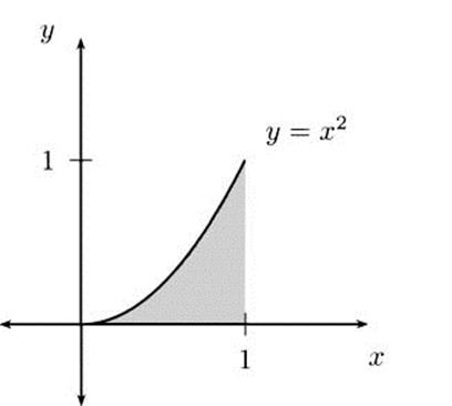
We would like to be able to find areas of many curved regions. For instance, what is the area under the function y = x² as x goes from 0 to 1? This is the shaded area in Figure 4.30.

We can see right away that whatever the area under the curve is, it must be less than 1, since the shaded region fits entirely inside a 1 × 1 square. In fact, it fits entirely inside a triangle with vertices at (0,0), (1,0), and (1,1), so the area must be less than 1/2.

Can we say what the area must be bigger than? A rectangle with vertices (0.5, 0), (0.5, 0.25), (1, 0.25), and (1, 0) fits entirely within the shaded region, and the rectangle has area 1/8, so we know the area must be larger than that.

There is a standard (clever) way to estimate unknown areas using shapes that are easy to understand, and it works much like the exploring we are doing here. You find easy-to-compute areas that contain your region and you find easy-to-compute areas contained entirely inside your region. The answer you desire must be somewhere in between. We always make our easy-to-compute areas from rectangles.

Figure 4.30 The area under x²

For example, divide the interval [0,1] into five congruent subintervals, at the values x₀ = 0, x₁ = 0.2, x₂ = 0.4, x₃ = 0.6, x₄ = 0.8, and x₅ = 1.0. In each little interval, find the largest value of the function f(x) = x². For example, on the interval [0,0.2] the highest value of the function is f(0.2) = 0.2² = 0.04. Use that highest value to create a rectangle, as in Figure 4.31.

Figure 4.31 Rectangles that fit over the function y = x².

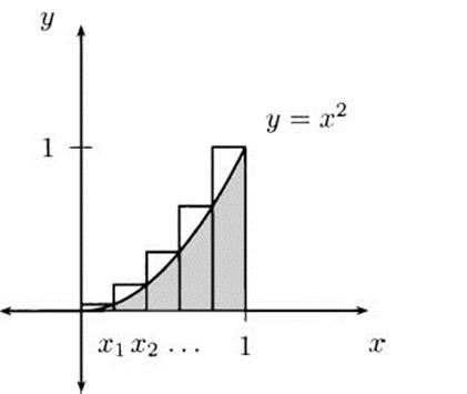
We can tabulate an (over-)estimate for the shaded area:

A collection of rectangular areas, summed to estimate the area of a curved region, is called a Riemann sum, after the German mathematician Bernhard Riemann (1826–1866). Riemann is famous, not only for his work on calculus, but for work in number theory (where the Riemann hypothesis is well known) and for foundational work in the mathematical branch now known as Riemannian geometry.

Notice that this Riemann sum comes to a bit less than 0.5, which was our first over-estimate for the shaded area. You can probably imagine what would happen if we were to use more rectangles. With 10 rectangles, we get an estimate for the area of 0.385 (check for yourself; the calculation is not difficult). As we use more and more “upper” rectangles, the estimates will continue getting lower and lower, becoming closer and closer to the area we are interested in.

Figure 4.32 Rectangles that fit under the function y = x².

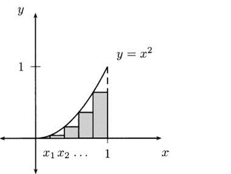
We can do something similar with rectangles lying under the curve, as in Figure 4.32. For example, in the subinterval [0,0.2], the smallest value of the function y = x² is 0. The only rectangle that could fit “under” the curve is a flat line, with no area at all. On [0.2,0.4] the smallest value of the function is 0.2² = 0.04. As before, we can tabulate an estimate of these “lower” rectangles:

As we did with upper rectangles, we can use more and more lower rectangles to get better (under-)estimates for the area. For example, 10 rectangles yields an area estimate of 0.285 (check for yourself).

Although we can get as close as we like, no finite number of upper or lower rectangles will exactly measure the area we want. Fortunately, there is a deep connection between derivatives and areas.

Fundamental Theorem of Calculus. Let f(x) be a continuous function over the closed interval [a, b]. If F(x) is any function with F′(x) = f(x), then the area under f on the interval [a, b] is F(b) – F(a).

EXAMPLE 4.41

What is the area below the function f(x) = x² on the interval [0,1]?

Solution: The Fundamental Theorem of Calculus tells us that to compute this area exactly, we only need to find some function F(x) whose derivative is x². The function works. Once we find F, we evaluate it at the ends of the interval and subtract, so the area is F(1) – .

Notice that 1 /3 is between the lower and upper estimates that we computed earlier using lower and upper rectangles.

EXAMPLE 4.42

What is the area below the function on the interval [0,2]? See Figure 4.33.

Figure 4.33 Area under from 0 to 2.

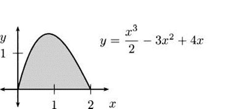
Solution: We need a function . If we take F(x) = – x³ + 2x², that works exactly. By the Fundamental Theorem, the area is F(2) F(0) = 2 – 0 = 2.

EXERCISES

4.79 Estimate the area under the function f(x) = x² on the interval [0,1] using ten equal subintervals and computing the Riemann sum using upper rectangles.

4.80 Estimate the area under the function f(x) = x² on the interval [0,1] using ten equal subintervals and computing the Riemann sum using lower rectangles.

4.81 The function F(x) = + 7 has the property that F′(x) = x². Use this fact to find the area under the function f(x) = x² for 0 ≤ x ≤ 1.

4.82 Let f(x) = x – 2.

a) Find a function F(x) whose derivative is f(x).

b) Find the area under the curve for 2 ≤ x ≤ 5.

c) Draw a graph of the function and find the area directly. (Hint: the region is a triangle.)

4.83 For each function f(x), find a function F(x) with F′(x) = f(x).

a) f(x) = x² + x + 1

b) f(x) = 4x³

c) f(x) = 4(x + 1)³

d) f(x) = 4(2x + 1)³

e) f(x) = e^3x+2

f)