Mathematics for the liberal arts (2013)

Part I. MATHEMATICS IN HISTORY

Chapter 4. CALCULUS

4.15 The Riemann Integral

Area is an important mathematical concept, and like other mathematical notions it has its own notation and careful definition. Informally, you can take the symbols

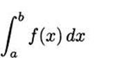
as representing the area under the function y = f(x) between the values of a and b. In words we read this aloud as “the integral from a to b of f of x dee-ecks.”

We call such an integral a definite integral, since it is defined on an actual (definite) interval [a, b]. The numbers a and b are called the lower limit and upper limit of the integral, respectively. Computing this area is “finding” or “taking the integral of f.” The process of finding an integral is called integration.

In the last section, we took for granted that we could find the area under a curve such as y = x² or y = sin x and then started looking at rectangles. But mathematicians are typically too careful to assume an answer will exist because it looks good in a picture. Mathematical objects can be surprisingly subtle. (For example, there is an object that has a finite volume and an infinite surface area. If you are curious, you may want to research Gabriel’s Horn or Torricelli’s trumpet.)

So, while we started with the intuitive idea of area and explored it by looking at rectangles, it turns out that mathematically that it should work the other way around. Mathematically, there is no question that any interval [a, b] can be divided into subintervals. Any function defined on an interval [a, b] can be evaluated at points of our choosing (including in each subinterval). So we can always form rectangles that match the height of a function in subintervals of [a, b].

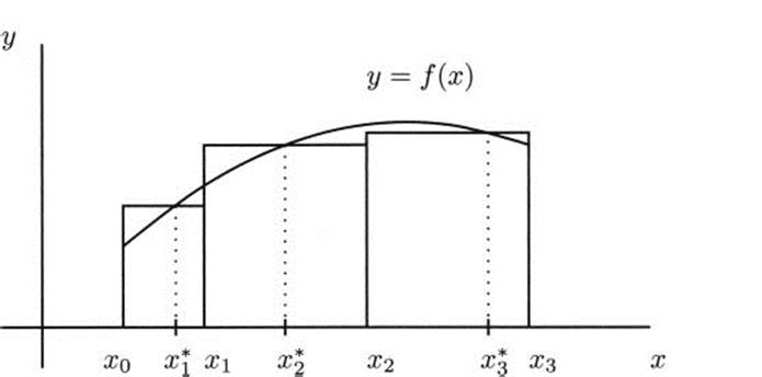
Figure 4.34 An area estimated by general rectangles.

While we can’t guarantee that our intuitive idea of area is correct, the process of taking rectangle estimates is completely rigorous. So this is actually how we define integrals (and we intuitively understand them to be areas). The definition of the Riemann integral is a limit of a sum of rectangles.

We have a lot of freedom about how we choose our rectangles. For example, it is convenient for all the rectangles to have the same width, but that is not necessary. In Figure 4.34 we can see an estimate made with three non-uniform rectangles.

The points that set the heights of the rectangles can be the left endpoint of each subinterval, or the right endpoint, or the midpoint. In fact, when you use more and more rectangles (when you take a limit), it doesn’t matter what point in each subinterval you use to set the height of the rectangle. We don’t even have to choose the same way in every interval, we just need some point in each interval. It has become convention to use “star” notation to indicate this. The value can be anywhere in [x₀, x₁]. In general, can be anywhere in the zth interval, [x_i–1, x_i].

In Figure 4.34 the height of the function at would be written f(), so the area of the first rectangle is height × width = f()(x₁ – x₀). The areas of the other rectangles are computed similarly, so the entire area estimate with all three rectangles would be

As we use more and more rectangles, the sums become tedious to write, so we usually use some abbreviation. We write Δx_i for the quantity x_i – x_i–1, which is the width of the ith subinterval. This makes our sum simpler:

In general, an area estimate with n rectangles looks like

Finally, as we use more (progressively narrow) rectangles, the area estimates often approach a single value. Another way to say this is that the sums have a limit as n (the number of rectangles) approaches infinity. Mathematically, we use this limit to define the integral:

In plain English, a Riemann integral is defined to be the limit of sums of (very narrow) rectangles. If the sums converge to some answer, then we define that to be the integral and refer to it as the area under the curve.

When you understand that the integral is defined in terms of sums, the notation for an integral makes more sense. It is an elongated ‘S’, standing for “sum.” Gottfried Wilhelm Leibniz (1646–1716) introduced the concept of the integral, and the notation, but it was Bernhard Riemann (1826–1866) who defined the integral formally and rigorously.

With this new notation, we can restate the major theorem we use to compute integrals, the Fundamental Theorem of Calculus, expounded by Barrow, Leibniz, and Newton:

Fundamental Theorem of Calculus. Let f(x) be a continuous function over the closed interval [a, b], If F(x) is any function with F′(x) = f(x), then

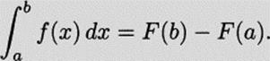
The function F(x) in the Fundamental Theorem is called an antiderivative of f(x). We say “an” antiderivative instead of “the” antiderivative, because antiderivatives are not unique. For example, F(x) = x² and F(x) = x² + 14 are both antiderivatives of f(x) = 2x.

The more antiderivatives we are able to compute, the more integrals we can find. That makes antiderivatives and antiderivative formulas important to us. It also means that we’ll want a notation for antiderivatives.

Definition. For a function f(x), the symbol dx represents an antiderivative of f. It is also referred to as the indefinite integral of f.

Even though we say “the” indefinite integral, we must remember that a function has many antiderivatives. Sometimes we refer to the general antiderivative by giving a formula for all of these antiderivatives at once. For example, the general antiderivative of f(x) = 2x is F(x) = x² + C, where we understand C to be any constant.

Integral Rules

Many of the derivative rules that we studied in Sections 4.5–4.7 have corresponding antiderivative (integral) rules.

The power rule: If n ≠ – 1, then

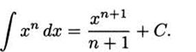
For example, x⁶ dx = x⁷/7 + C.

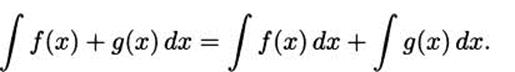
There are also an integral sum rule and a constant coefficient rule.

The sum rule: The integral of a sum is the sum of the integrals:

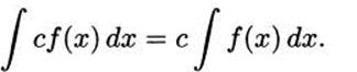
The constant coefficient rule: If c is a constant, then

EXAMPLE 4.43

Find the general antiderivative of the polynomial f(x) = 12x³ – 5x² + 1.

Solution: If we carefully apply the preceding rules, we get

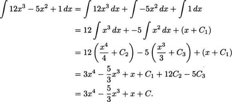
In the last line of our calculation, we recognize that C₁, C₂, and C₃ are all constants, and a sum of different constants (even when scaled by multiplying or dividing by some fixed number) is merely another constant.

We can easily check that we are correct. If we take the derivative of our answer, we get f(x) back.

EXERCISES

4.84 Find each indefinite integral (general antiderivative).

4.85 Find each area