Mathematics of Life (2011)
Chapter 14. Lizard Games
A male lizard has secured himself a female, and soon the pair will mate. She seems to like his sky-blue throat, and the two of them are often seen walking out together. But suddenly this lizard equivalent of marital bliss is shattered by an intruder. He is bigger and stronger than the blue-throated lizard, and his throat is orange. He threatens the blue-throated lizard, hoping to drive him away and steal his female. When the blue-throated lizard resists, the orange-throated one attacks.
This turns out to be a tactical error on both their parts, because while they are engaged in battle, a smaller lizard with a yellow throat sneaks up on the female and mates with her.
This reptilian soap opera is played out over and over again on some of the many islands that dot the western coast of North America. Since the males are competing for the same female, we would expect them all to belong to the same species, and despite their different colours, they do. The males are different ‘morphs’ – types – of the common side-blotched lizard, scientific name Uta stansburiana.
Their Heat-magazine-style mating strategies have remarkable consequences.
Barry Sinervo, working from his lab at the Department of Ecology and Evolutionary Biology at the University of California in Santa Cruz, has been following the patterns of heredity in one population of common side-blotched lizards since 1989. Because they live on the same island and interbreed, they can be assigned to a single species with some confidence. As we have just seen, the males of this species occur in three distinct morphs, and the main distinguishing feature is the colour of the lizard’s throat, which can be orange, blue or yellow. The three morphs also differ in size, with the orange-throated ones tending to be larger and the yellow-throated ones smaller.
These colours seem to be an example of what Darwin called sexual selection: they relate not to general survival characters, but to female preferences when choosing mates. Anything that the ladies prefer tends to become more common, because it gets passed to their offspring. The peacock’s gigantic, brightly coloured tail and the gaudy and bizarre decorations of birds of paradise are familiar examples.
Year in, year out, each morph follows its own particular mating strategy. Blue-throated male lizards form strong pair bonds with their females; orange-throated and yellow-throated ones don’t. Orange morphs, which are the strongest, fight blue ones and take away their females. Yellow ones are coloured much like females, and thanks to this disguise they can take advantage of fights to approach without causing alarm, and mate with the disputed female. The blue ones rely mostly on strong pair bonding, tend to lose out to the stronger orange ones, but can defeat the yellow ones. In simplified terms:
• orange beats blue,
• blue beats yellow,
• yellow beats orange.
So orange is fitter than blue is fitter than yellow is fitter than ... orange. So much for ‘survival of the fittest’.
What on earth is going on here? How does this evolutionary competition pan out, and how does it fit into a Darwinian picture?
One of the biggest problems with the theory of evolution is that everyone thinks they understand it. But it would be much fairer to say that no one understands it – not even evolutionary biologists. Evolution is extremely complex and extremely subtle. It is not just a matter of the ‘best’ or ‘fittest’ creature winning the battle for survival. If it were, then one colour of male common side-blotched lizard would have displaced the other two long ago.
Is this a sign that, for these lizards, evolution doesn’t work? It certainly looks that way if you take the slogan ‘survival of the fittest’ literally and interpret it naively. Even if these lizards’ strange mating habits did evolve, they make it clear that the slogan is not a very good one. For this kind of reason, biologists avoid it.
Survival as such is not the main criterion for natural selection to operate: what counts is whether a creature manages to breed. It obviously has to survive to breeding age if it is going to have any chance of breeding, but it may fail to breed even if it has survived. The lizards demonstrate this point admirably. In innumerable species, only a few males breed, and they spend much of their time fighting the others to protect their own conjugal rights.
Moreover, the concept of ‘fitness’ in evolution is slippery. It’s not just a matter of assigning a fixed measure of fitness to each creature, and comparing the numbers to determine which one will out-compete the other. If it were that simple, the planet would end up with exactly one species: the fittest one. But life on Earth is not like that. Natural selection is not like that either, and neither is biological fitness.
Evolutionary biologists have a love – hate relationship with fitness. They are aware of its shortcomings, but some of them feel that if these can be circumvented, the concept adds predictive value to evolutionary theory. What quickly becomes clear, if you follow that line of thought, is that the fitness of an organism does not depend just on the organism: it also depends on the context. In a game of golf, Tiger Woods would be fitter (much fitter) than me, but in a game of mathematics I would be fitter than Tiger. Paula Radcliffe would be fitter than either of us if we were running a marathon. What makes organisms ‘fit’ depends on which game is being played, as well as on the organisms playing it.
If we insist on understanding the behaviour of the three lizards in terms of some concept of fitness, tailored to their particular games, then the definition of fitness must depend on which game the creatures are playing. Yellow-throated males will lose out against orange-throated ones in a straight fight, but they can win if the orange-throated one is distracted by a battle. The blue-throated lizards’ devotion to their mates will defeat the yellow-throated lizards, but not the orange. And the orange-throated lizards can beat the blue-throated ones in a fight, but they have difficulty keeping an eye on those sneaky yellow-throats.
I referred to the lizard soap opera as a game – and so it is, in two senses. First, it has a lot in common with a game that children like to play. Second, both the lizards’ game and the children’s one can be modelled by a specific mathematical process, which happens to be called a game. Accordingly, the relevant area of mathematics is called game theory.
The childhood game I have in mind is scissors – paper – stone. Each player holds one hand behind their back and chooses either scissors, paper or stone by appropriate placement of the fingers: two separated fingers for scissors, flat palm for paper, clenched fist for stone. The payoffs (wins and losses) are governed by the rule that scissors cuts (beats) paper, paper wraps (beats) stone, and stone blunts (beats) scissors. Suppose Alice and Bob play, with Alice going first. With a point score of 1 for a win, -1 for a loss and 0 for a draw, the table of payoffs for Alice (technically called the payoff matrix) is as shown in Figure 58. The payoffs for the second player are the same, except 1 and -1 are swapped. That is, if Alice wins then Bob loses, and conversely.
Intuitively, scissors – paper – stone is fair: neither player has a clear advantage. This would not be the case if, to take an extreme example, the payoffs were such that Alice always wins, with 1’s everywhere. In fact, scissors – paper – stone is symmetric: it treats both players equally. I won’t formalise this idea of symmetry – it can be done, but it’s technical and doesn’t have a lot of content – but whatever move Alice chooses, Bob has a choice of one winning move, one losing move and one move that leads to a draw. So there is no bias against Bob. By the same argument, there is also no bias against Alice. We therefore expect that in the long run neither player will come out ahead to any significant degree. This turns out to be true, as long as the players don’t introduce a degree of bias by making ‘bad’ choices.
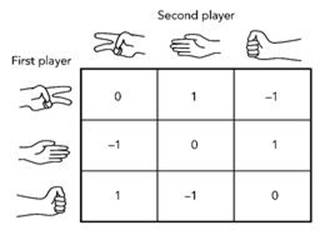
Fig 58 Table of wins (1), losses (-1) and draws (0) for the first player in scissors – paper – stone.
Suppose, for instance, that Alice chooses scissors significantly more often than paper. Then Bob may notice. If he does, he could choose stone on every play and come out ahead, because in that case Bob wins whenever Alice chooses scissors, loses when she chooses paper and draws when she chooses stone. So Bob will win in the long run. In practice, if Bob’s strategy were that obvious, then Alice would notice and start playing paper every time instead. However, the same reasoning applies if Bob makes random choices, but biases them in favour of stone: he will come out ahead if Alice favours scissors.
Pursuing this analysis leads to the reasonable conclusion (also a consequence of symmetry) that Alice should choose each possible move at random, with probability 1/3. Bob should do the same. Indeed, if one player departs from such a strategy, either by introducing regular patterns such as alternating paper with scissors, or by using probabilities that differ from 1/3, then the other player can find a response that wins in the long run.
Scissors beats paper beats stone beats scissors ... Familiar?
Orange beats blue beats yellow beats orange.
Could the common side-blotched lizards’ mating games somehow be analogous to scissors – paper – stone? And if they were, what would that tell us?
The great Hungarian-American mathematician John Von Neumann was one of the father figures of computing and a polymath who ranged over many areas of mathematics. A child prodigy born into a Jewish family, he spent four years teaching at the University of Berlin, and then went to Princeton University in the USA. When the Institute for Advanced Study at Princeton was created in 1933, he was one of the founding professors. Another was Albert Einstein. In 1927, having turned his mind to economics, Von Neumann invented a new branch of mathematics: game theory. A year later he made a fundamental discovery, the minimax theorem. Further developments led to the 1944 Theory of Games and Economic Behavior, written with Oskar Morgenstern, which hit the front page of the New York Times.
A game, in Von Neumann’s sense, is a simple mathematical model of two (or more) competing players, each faced with various choices, in which the payoff to each player depends on the combination of choices that they make. The players are assumed to know the table of payoffs, but have no knowledge of their opponents’ choice. The game can be played just once, in which case we have to analyse the probability of winning or losing, or it can be played many times, in which case we can analyse the frequency of winning or losing (and how much is won or lost). A basic theorem in probability theory, the law of large numbers, says that in the long run the frequencies ‘almost always’ give the probabilities, so the two ways of thinking are mathematically equivalent. The usual choice is to consider what happens when the game is played many times, because our intuition for this is better than our intuition for one-off probabilities.
Scissors – paper – stone is a typical game, with one exceptional feature: its threefold symmetry. Most games treat different combinations of players in different ways. For instance, in the hawk – dove game, the players are in contention over some resource. Hawks always choose to fight, and escalate the battle until either they are injured or the other player breaks off the engagement. Doves always retreat from hawks. Depending on the entries in the payoff matrix, there can sometimes exist mixed strategies in which the best way to play is to switch randomly from hawk to dove and back again with particular probabilities.
Game theory first took off in 1928, when Von Neumann proved the minimax theorem. This states that in a particular class of twoperson games with a very simple structure, there always exists a mixed strategy that permits both players simultaneously to make their maximum losses as small as possible. But this discovery was only the beginning. Another important piece of the puzzle fell into place when John Nash, the subject of the book and movie A Beautiful Mind, made a fundamental breakthrough for games with many players. He defined the concept of a Nash equilibrium and proved that one always exists. A set of players is in Nash equilibrium if each member of the set is making the decision that is best for them, given the decisions that the others have made. This is a sensible candidate for a rational strategy.
The person most responsible for the systematic application of game theory to evolutionary biology is John Maynard Smith. In 1973, in collaboration with the London-based American population geneticist George Price, he put forward one of the most important concepts in the field: that of an evolutionarily stable strategy. This is a refinement of a Nash equilibrium, and it pins down the conditions under which no mutant can successfully invade a population: a type of evolutionary stability.
Imagine a population of organisms, all of which have adopted – evolved – a particular survival strategy. In a genetic interpretation, this strategy will be inherent in their genes, as a result of many generations of natural selection. The organisms will not be consciously aware that they are adopting a strategy; it will simply be something that they do naturally, which has evolved because it works. Now suppose that there is some kind of genetic mutation, so that a similar organism, with a different strategy, suddenly appears in their midst. Can the mutant successfully establish a lineage of surviving descendants, or will it be weeded out by natural selection?
For example, consider the hawk – dove game in the trivial case where the population consists only of doves. This is not an evolutionarily stable strategy, because any hawk mutant can successfully invade – hawk always wins against dove. That is, hawk receives a positive payoff, while dove gets zero.
Maynard Smith devised a mathematical definition of an evolutionarily stable strategy. Suppose there is a finite list of available strategies. Let E(A, B) be the payoff to an individual who adopts the original strategy A against an opponent who adopts strategy B. This is an entry in row A and column B of the payoff matrix.
Before the mutant appears, there is only one game in town: the entire population is playing the same Old strategy, and the payoff to each individual is E(Old, Old). When the mutant appears, it adopts a strategy New. The payoff to the mutant is then E(New, Old). If E(Old, Old) is greater than E(New, Old), then the mutant will lose the competition against any member of the original population, so its lineage will be weeded out. There are two other possibilities: either E(New, Old) is greater than E(Old, Old), or the two are equal. In the first case, the mutant wins and its lineage survives: it has successfully invaded the population. In the second case, the mutant loses out if the original strategy Old has a greater payoff against New than New does against itself; that is, if E(Old, New) is greater than E(New, New).
The Old strategy is said to be evolutionarily stable if no mutant can successfully invade.
Some games have evolutionarily stable strategies, others do not. A general payoff matrix for two strategies Old and New looks like this:
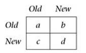
An evolutionarily stable strategy exists provided a is smaller than c, and d is smaller than b. The strategy concerned adopts Old with probability (b-d)/(b+c-a-d), and New with probability (c-a)/ (b+c-a-d).1
When applying these models to real examples, the main difficulty is to estimate the entries in the payoff matrix. In principle, they could be estimated by playing one strategy against another many times and seeing what happens on average. But in practice this may not be possible. Suppose, for instance, that we are trying to understand some stage in the evolution of dinosaurs. We can’t pit dinosaurs against one another and see who wins. So the entries have to be estimated on the basis of other factors.
Game theory sheds light on the evolution of new species, which can arise when changes in the environment render a single-species strategy evolutionarily unstable. If so, then a mutant can successfully invade – and given enough time, a suitable random mutation should arise. This doesn’t explain speciation, but it does determine circumstances under which it might or might not be possible.
Darwin titled his book The Origin of Species. Biologists have built on its main ideas ever since. So can you guess what is one of the biggest mysteries in evolutionary biology today?
That’s right. The origin of species.
However, that does not mean that Darwin was talking nonsense and species have not evolved. It reflects the difficulty of reconstructing fine details of processes that occurred millions or billions of years ago, and the rich complexity of today’s living world. This is hardly surprising. What is surprising is how strong the evidence for evolution is, and how much we already know about it.
You may wonder how scientists can be sure that evolution has happened when they don’t understand many of the details. However, we are faced with exactly this situation on a regular basis. We know that our child has learned things at school, but we weren’t in attendance ourselves. We know that he or she has learned to speak, requiring changes in the child’s brain, but we don’t have high-resolution before and after brain scans to prove it. We know that the cat brought a mouse in last night, because the gruesome evidence is on the kitchen floor, but we never saw the cat do it. Science is seldom about direct observation: it is nearly always about indirect inference.
We know that evolution has occurred throughout the history of life on Earth because many independent lines of evidence attest to the general nature of the process. Some of this evidence has survived for millions of years. We can measure the sizes of fossil horses, correlate them with the ages of those fossils as determined by the geological strata in which they are found, and see a slow but steady trend towards larger and larger animals. But if we want proof that two particular horses were competing with each other at some particular instant of time, say 10.34 in the morning on 16 April 18,735,331 BC, then nothing short of a time machine would enable us to observe the competition directly. Instead, we infer that in general terms the horses were competing with each other, because it is very hard to see how they could have avoided competing. Population growth, if unchecked, would soon have caused horses to overrun the entire planet. So something must have checked it, and virtually any such process is a form of competition.
Were they competing for access to females? For food? What kind of food? Why didn’t those two horses have enough for both of them? Which one won? When the required level of detail gets too high, there is no serious chance of answering such questions.
Not only are we unsure of many details of the evolution of species, but we don’t really have a good definition of what a species is. Again, that does not mean that blackbirds cannot be distinguished from whales. But certain fine distinctions are difficult to pin down precisely. Ironically, this very difficulty supports the theory of evolution: if species are not always discrete, separate groups, then it is easier to see how natural selection might cause new species to split off from old ones.
You might think that ‘species’ must have a straightforward definition. After all, taxonomists classify organisms according to which species they belong to. In the Linnaean scheme, you and I belong to the species Homo sapiens, my cat belongs to the species Felis catus and the silver birch tree in the garden belongs to the species Betula pendula. This shows that particular species can be defined, but it no more tells us what a species is than the list ToyotaAvensis, Ford Mondeo, Volkswagen Golf tells us what a model of car is.
One of the most popular definitions of species was advocated by the German-American ornithologist Ernst Mayr: species are groups of interbreeding natural populations that are reproductively isolated from other such groups. This definition applies only to sexual organisms, because ‘interbreed’ requires sex. As a working definition – a guideline that works fine most of the time – it is pretty good. However, it has a few drawbacks if it is taken literally and expected to apply in all cases.
For instance ... There is a chain of gulls, more or less continuous, that begins in Britain, goes right round the world, and ends up close to where it started. At one end are herring gulls; at the other, black-backed gulls. These two types of gull satisfy Mayr’s definition: they do not interbreed, hence are ‘reproductively isolated’. They look different, and they are different. They both coexist (without interbreeding) in Britain: mixed urban colonies are found in Bristol, Gloucester and Aberdeen. However, along the chain, each group of gulls can and does interbreed with its neighbours. So by that same definition, all neighbours belong to the same species as each other. Therefore herring gulls and black-backed gulls must also belong to the same species. But they don’t. It’s like a string of beads, each one the same colour as its immediate neighbours, but with black at one end and white at the other.
An enormous variety of alternative definitions of ‘species’ have been proposed over the years. Mayr’s remains popular, but there are circumstances in which it seems inappropriate: the gull story is far from unique. Alternatives to interbreeding include the potential to exchange genetic material, genetic similarity, morphological similarity, ecological similarity, common ancestry and technical ideas in cladistics.
Massimo Pigliucci is a biologist at Lehman College in New York whose background includes genetics, botany, ecology and – unusually – philosophy. He analysed the different definitions of speciation in the literature, and found all of them lacking. Just as Mayr’s proposal is confounded by an arc of gulls, so each of the others fails to match some aspect of the rich and messy reality of biology. On the other hand, each works pretty well within a limited domain and for specific purposes. Pragmatically, that might be considered good enough: this is the empirical view that ‘species’ is a convenient way to distinguish organisms, and criticisms of any particular definition are mostly linguistic nitpicking. But that doesn’t answer a basic question: is ‘species’ a fundamental level of organisation of the biological world, or is it an artificial classification scheme foisted on us by taxonomists, with no real significance for actual organisms? Pigliucci puts it like this:
The so-called ‘species problem’ is one of those topics of discussion among evolutionary biologists that has been present since before Darwin’s publication of the aptly titled Origin of Species (Darwin himself referred to it as an already old problem) and will probably never go away ... On the one hand, [biologists] tend to turn away in disgust when species concepts are brought up by colleagues, are the subject of papers, or are discussed at conferences. On the other hand, they simply cannot resist the temptation to offer graduate seminars on the topic and avidly read anything that is published on the subject.
Many biologists consider the whole issue to be merely one of semantics – finding an acceptable definition for practical purposes, which matches empirical observations in the field. Pigliucci argues that the problem goes deeper, with ‘strong philosophical overtones’. He discusses three main themes that dominate the philosophical literature on the problem: critiques of definitions proposed by biologists, analysis of what kind of thing a species is (individual? group? natural type?) and the possibility that more than one concept of species is needed anyway, depending on context and purpose. The solution he proposes is founded on the philosopher Ludwig Wittgenstein’s idea of ‘family resemblance’. The family resemblance, he suggests, is real: it has biological significance, and is not just a human invention that provides neat lists of types of organism. However, by its nature it is difficult to pin down a simple, neat, tidy definition that characterises this kind of family resemblance.
Here is Pigliucci’s main conclusion, rephrased in terms congenial to a mathematical biologist. First, we exploit the idea of multidimensional spaces to represent a list of phenotypic (and/or genotypic) data as a point in a conceptual space of many dimensions. Call this phenotypic space. Then we plot the points that correspond to each organism under investigation. We also need some notion of how far apart or close together two organisms are. There are many ways to set up such a ‘metric’ – by measuring the differences in characters such as wingspan or beak size, by comparing gene sequences, by looking at patterns of behaviour – what food do they eat? – and so on. A cluster is then a collection of data points in phenotypic space whose members are closer to one another than they are to anything else. What emerges from this viewpoint is that a satisfactory definition of species is elusive because a definition of cluster is elusive – it depends on the choice of metric, for instance. That’s Pigliucci’s philosophical point. The distribution of organisms in phenotypic space is not a convention: it is real, and can be observed. The problem is how to break the distribution into clusters, and what that is taken to mean. On the whole the answer is usually fairly obvious, which is why all the traditional definitions work pretty well, most of the time. When they don’t, there are two ways to proceed: tinker with the metric, or refine the definition of a cluster.
A key feature of this proposal, says Pigliucci, is that it stops biologists ‘wasting their time by trying to empirically solve a problem that has philosophical components that cannot be settled by the accumulation of new data’. Collecting vast quantities of data about, say, the disputed taxonomy of lizards living on islands down the west coast of North America will never resolve the taxonomic issues, which are really about the choice of metric and the concept of cluster involved. However, such data may contribute to the analysis of the situation when the metric and concept are chosen, and could even guide their choice.
Looking for clusters within data may sound vague and woolly, but there is an entire branch of statistics devoted to the topic: it is called cluster analysis. As with any well-developed branch of mathematics, cluster analysis applies many different methods to the same general class of problems, and which one works best depends on the problem. I’ll concentrate on the simplest method. In practice it is performed using algebraic calculations on numerical data, but the underlying idea is easier to understand in visual form.
Suppose that a field ornithologist on some exotic island is observing birds. One thing they might do is capture birds, measure various characters and record the measurements. For efficiency, they would probably record several dozen characters, but to keep the explanation simple and make it possible to draw pictures, I’ll consider just two: beak size and wingspan. It doesn’t actually matter what these variables represent: just that for each individual bird the ornithologist gets two numbers. Having collected the data, the ornithologist plots them on a diagram, which might resemble Figure 59, where I’ve used made-up data for illustrative purposes. I’ve also omitted scales from the axes.
The left-hand graph shows the plotted data. It’s difficult not to notice that the points form two distinct clusters. The clusters might correspond to two distinct species, or perhaps two subspecies within a given species. Which of these is appropriate depends on the level of detail: how wide the square is relative to the numbers that constitute the data. If it’s a big square, then birds in one cluster are significantly different from those in the other cluster, and the clusters represent species. If the differences in data are just a few per cent, we might be talking about subspecies.
As well as the two clusters, a single point lies on its own at lower right, and it’s not clear whether it belongs to the cluster to its left, or is part of a third cluster. Such points are known as outliers because they are rare exceptions to the overall pattern. The method of data analysis means that their effect is small, and it makes little difference to the results if they are discarded. But this point might also represent a new, rare species, so in practice it would be better to collect more data.
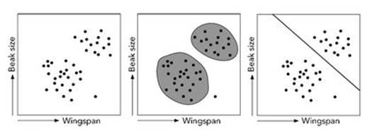
Fig 59 Left: Data. Middle: Two clusters and an outlier. Right: Separating the clusters.
The eye easily separates the data into two clusters, but it is not straightforward to program a computer to perform such a task. The simplest form of cluster analysis seeks to separate the data into two subsets by, in effect, drawing a line between them. More precisely, the method sets up some combination of the two variables, such as
0.5×(wingspan) + 7.3×(beaksize)
together with a threshold value, say 15. Any choice of these three numbers splits the data into two subsets: one consisting of data for which the combined value is greater than the threshold, the other consisting of data for which it is smaller. If these numbers are chosen correctly, then the two subsets will be widely separated, but within each separate subset the numbers will be much closer together. All of this can be made precise, and carried out as a numerical calculation.
Figure 60 shows real data for the horned beetle Onthophagus nigriventris. The two variables plotted are body size (horizontal axis) and length of horn (vertical axis). The open circles are males, the black ones females. Ignoring this distinction, the most obvious clusters are all the females together with some of the males, and the rest of the males. The two are clearly separated – for example by a horizontal line drawn through horn length 7 mm.
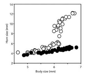
Fig 60 How the beetle changed its horns. Relation between body size and horn length for males (open circles) and females (solid circles) in the horned beetle Onthophagus nigriventris.
If we introduce a third variable, sex, plotted in a third dimension, then the males and females are immediately separated, making the point that extra data measuring new phenotypic variables can dramatically change the clusters. Since the distinction between males and females is standard, and we expect significant phenotypic differences between the sexes, it is a reflex to separate the data by sex – hence the two colours of dots.
The males here all belong to the same species, even though they are split between two clusters. In particular, they can all interbreed with the same females, and the females form one cluster. Nonetheless, the males clearly do split into two clusters, and recording extra variables can only reveal further splits, if there are any. These clusters represent two different morphs – phenotypes that have evolved according to two distinct strategies within the same population. Some males, called majors, go for big horns and an aggressive personality. They employ their large horns to fight other males, for access to females. The evolutionary advantage of this strategy is clear: the bigger your horn, the more formidable you are in combat. The other males, minors, develop rudimentary horns and avoid combat. Experiments suggest that one advantage of this strategy is greater manoeuvrability in tunnels. But it might allow the minors to sneak up on females while the majors are having their fights, because minors resemble females a lot more than they do majors.
This kind of separation of mating strategies occurs in the males of many species; we’ve already seen it in lizards. It is particularly extreme in horned beetles. It might be a sign that the species is in the process of splitting.
The use of straight lines, or their equivalents when there are more variables, avoids the trap of using ever more complicated formulas to model data. This can lead to an almost perfect fit between data and model, but one that is entirely meaningless. However, sometimes there are genuine clusters, but no straight line can separate them. Think of a tight circular cluster surrounded by a larger horseshoe-shaped one, for instance. Clusters like these can be detected by allowing nonlinear terms in the algebra – such as the square of the beak size or the beak size times the wingspan.
Recall that the divergence of a single species into two (or perhaps more) distinct ones is called ‘speciation’. Evolutionary biologists recognise many types of speciation, but there are two main ones: allopatric and sympatric. The words are derived from Greek: allos=other, sym=together, patra=homeland. Speciation is allopatric if it takes place in different locations, in a specific sense that I will explain in a moment, and sympatric if it takes place in the same location – also in a specific sense.
The big issue in speciation is not the potential for a group of more or less identical, happily interbreeding organisms to diverge. Well before Darwin, everyone knew that descendants are not identical to their ancestors, and the breeding of domestic animals showed that the same kinds of ancestor can give rise to very different descendants. For instance, a breed of sheep with short wool might occasionally have offspring with long wool, or wool of a different colour. In this instance, human intervention can persuade the sheep population to realise that potential, but the new types of sheep are not new species, just new breeds. Nevertheless, the potential to diverge must have been present. For true speciation to occur, whether by human hand or by unaided nature, the problem is to keep the new types separate. Otherwise they may interbreed, and then they are likely to reconstitute the original stock.
Somehow, the two diverging groups must be reproductively isolated.
Traditional methods of animal breeding achieve this by direct intervention: the breeders control which animals mate with which. This is how breeds of pedigree dog are maintained, and one of the reasons why they are so expensive. Distinct breeds of dog, left to their own devices, would revert to a population of mongrels within a few generations.
Allopatric speciation achieves the same result through some form of geographical isolation (‘different homeland’). The idea is that some natural feature, such as a river, a mountain range or a land bridge, separates what was initially a single population into two distinct ones. Once separated, the two groups can change, and they are likely to do so in different ways because they have ceased to interact with each other. If this process continues for long enough, it may become impossible for members of the two groups to interbreed. At that point, the groups constitute distinct species.
Here’s a classic example. The Caribbean Sea just north of the Isthmus of Panama, and the Pacific Ocean to its south, contain many organisms that are closely related but constitute distinct species. Working from the Scripps Institution of Oceanography in San Diego, the marine biologist Nancy Knowlton has studied snapping shrimp.3 Very similar species of shrimp – they look almost identical – are found on both sides of the isthmus, but when brought together they do not interbreed. Every single one of seven distinct lineages of snapping shrimp has split into two species (in three cases there is also a third subspecies): one branch lives in the Caribbean, the other in the Pacific (see Figure 61).
It is straightforward to provide an evolutionary explanation, and difficult to find anything else that makes sense of this remarkable pattern. We know independently from geological evidence that three million years ago falling sea levels and rising land filled in the gap between the two halves of the American continent, creating the Isthmus of Panama and separating the Pacific Ocean from the Caribbean and the rest of the Atlantic. Before the land bridge formed, each lineage constituted a single species. Afterwards, allopatric speciation caused each lineage to split into two (or more) species, the ones we have today. For each lineage, the modern species of snapping shrimp are descendants of the same ancient species, which ‘drifted apart’ genetically once the two populations were prevented from interbreeding by an impassable land barrier.
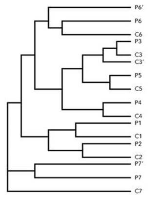
Fig 61 Family tree of snapping shrimp. Seven lineages, four pairs of species and three triples (including subspecies). P=Pacific, C=Caribbean. One species in each pair lives either side of the Isthmus of Panama.
This evolutionary hypothesis makes a quantitative prediction. If we can work out the time that has elapsed since the species began to diverge, independently of the geology, we should obtain a result of about three million years. The discovery of DNA has made such estimates possible, because mutations occur at an approximately constant rate.4 If the two times disagree, something is wrong. As it happens, they do agree.5 So here we have a specific prediction made by evolutionary theory and confirmed by experiment.
There are more ways to test the theory of evolution than watching a cauliflower and insisting that it must change into a cat before your very eyes.
The allopatric mechanism for speciation is simple and direct; computer scientists would call it WYSIWYG – what you see is what you get. To separate something into two parts when it wants to stick together, drive a wedge through it. Perhaps for this reason, most biologists believe that most speciation events have been allopatric, and they have found examples everywhere – the African and Indian elephant, squirrels on the two sides of the Grand Canyon, the Faeroe Island house mouse ...
As a mathematician, I tend to be suspicious of WYSIWYG explanations. They put in what they want to get out, which smacks of circular logic. The world is usually less direct. Sympatric speciation is definitely less direct, but it is also more puzzling. For a long time, it was thought to be exceedingly rare, if not impossible. Initially there is a single species, a group of more or less identical creatures (except for sex if the species is sexual). They are all able to interbreed with one another, with fertile offspring. They are all conveniently located in the same place, so there is no lack of opportunity to interbreed. Suppose that for some reason this single group starts to split into two or more genetically different types. Then there seem to be two immediate reasons why this split should not develop into a lasting division into two distinct, noninterbreeding groups, let alone two groups that cannot interbreed with fertile offspring – two distinct species.
One reason is genetic. In the early stages of the split, the two new types can interbreed and there is no geographical barrier to stop them. Because the new types are small in number but the main population is large, the mates of the new types will almost always be members of the main population. But then, the new genes will be overwhelmed by the existing ones. So as soon as a group begins to acquire genetic differences, those changes will be snuffed out – swamped by the main gene pool – and the result recreates the genetic make-up of the original species.
This is the problem of ‘gene flow’. It presents a stabilising force that mitigates against sympatric speciation.
Another objection is evolutionary. At least one of the new types differs from the original population. In order for this new type to evolve, creatures of that type must be fitter than the original population. But if belonging to the new type makes some particular creature fitter, then the same must apply to all the others. So why don’t they all change in the same way, thereby sticking together as a single species? The species might drift, as a whole, but it shouldn’t split.
I’ve already explained why the concept of ‘fitness’ needs to be treated with care, but the argument just outlined applies whatever specific meaning is attached to that term. It seems watertight. So it looks as though sympatric speciation is impossible. And that’s what most biologists thought until the last decade or so. Then a series of theoretical models and observations, mostly in laboratories but occasionally in the wild, made some of them rethink the whole question. And it has turned out that the arguments against sympatric speciation are not as strong as they appeared to be. Agreed, something has to stop gene flow from gluing the nascent split back together before it has really got going. But geographic isolation, as in the allopatric case, is not the only game in town. It is not necessary for organisms to be physically prevented from interbreeding. It is enough that, for some reason, they don’t.
A case in point is the (I say ‘the’, but see how the story goes) African elephant. When I was at school, we were taught that there are two species of elephant, African and Indian. Almost all taxonomists were happy with that, but for a century or so a few mavericks kept wondering about the forest and savannah elephants in Africa. No elephant can be called sylph-like, but forest elephants are significantly slimmer than savannah ones, and there are other differences in form and behaviour that suggested to these taxonomists that there must actually be two species of African elephant: forest and savannah. Nonsense, said the rest: the forests are adjacent to the savannahs, so the elephants in the forest can interbreed with those on the plains, and gene flow will do the rest. They may be distinct subspecies, but they can’t be different species.
The argument raged for a century, all of it inconclusive. Then, in 2001, Science reported that a DNA identification system, set up to trace poached ivory, showed that African elephants consist of two different species.6 The researchers were expecting slight variations between the genetics of forest and savannah elephants, consistent with their being subspecies, but the difference was much greater than expected. The DNA evidence showed that the species diverged about 2.5 million years ago. In fact, the genetic difference between the African forest and savannah elephants is 58% of that between either of them and the Indian elephant. So now most taxonomists accept that there are two elephant species in Africa: the forest elephant Loxodonta cyclotis and the savannah (or bush) elephant L. africana.
Why doesn’t gene flow reunite the populations into a single species, then? Although the forest is adjacent to the savannah, and it is true that elephants from the forest can mate with those from the plains, they seldom do. One reason is obvious: they don’t get much opportunity. A female and a male must come together accidentally at the forest edge, just when both are ready to mate – which in elephants is a fairly small proportion of the time. Even if they manage that, she has to fancy him, and often she doesn’t. So although their geographical ranges overlap, or at least abut, gene flow does not glue the two species back together.
Some taxonomists argue that the African elephant story is still allopatric speciation: in effect, the edge of the forest acts as a geographical boundary. But while they were arguing that there had to be just one species, thanks to gene flow disrupting sympatric speciation, this ‘boundary’ never figured in their arguments. Yaneer Bar-Yam has devised mathematical models based on genetic diffusion which show that gene flow can be prevented without having an impenetrable barrier.7 A sparsely spaced series of obstacles is enough.
We don’t know exactly how the two species of African elephant diverged. But if the distinction between allopatric and sympatric speciation means anything (and those who believed sympatric speciation to be impossible certainly thought it did), then the African elephants diverged sympatrically. Whenever a species starts to diverge, there will always be some sense in which one group is different from the other, otherwise there is no divergence. That difference may well affect the prospects of members of the two groups mating: not whether they can do so, but how likely it is that they will. On the other hand, whenever a species starts to diverge, the creatures will initially be in much the same location. So seizing upon some tiny difference and arguing that it constitutes allopatric speciation is really just renaming sympatric speciation.
The divergence of species involves the fate of individuals and their descendants, as well as family groups and the population as a whole. You don’t just wake up one morning to find two neatly separated groups of elephants, when the night before there was only one. From Massimo Pigliucci we have learned that ‘species’ is best seen as a particular scale of clustering in phenotypic space; in the same way, ‘speciation’ is a divergence of clusters on a similar scale. It starts with one cluster and ends with two, but could be very complex and messy in between. Mathematical models suggest that this may well be the case.
So sympatric and allopatric speciation are convenient broad categories, not mutually exclusive alternatives. As such they are useful because they capture a key difference: how the animals do or do not interact during the speciation process. Are they all in one place, or not? And the current view is that they may well be in the same place, so the speciation can be sympatric, while a host of influences can disrupt gene flow and allow the genetic and phenotypic split to grow. As the American geneticist and complexity scientist Stuart Kauffman put it at a conference in Sweden some years ago: the key step to speciation is getting a foot in the door. If that’s possible, then the door can be kept open, and maybe widened.
Darwin’s discussion of evolution is purely verbal, aside from one quasi-mathematical diagram, a tree-like figure showing how repeated small-scale branchings can combine to give large-scale divergence. But because evolution is a complex and sophisticated process, words alone are no longer adequate to describe it or debate it. Increasingly, the subject is being studied using mathematical models. The advantage of such models is that they make the assumptions involved clear. The disadvantage is that no model can capture the full complexity and vast scale of evolution, which has been going on in parallel across the entire planet for nearly four billion years.
Traditionally, biologists used that complexity as a reason to ignore mathematics and fall back on words. But verbal descriptions are even less able to capture the complexity of evolution than are mathematical models. Worse, they are imprecise and open to misunderstandings and ambiguities. The models clarify the concepts, the assumptions and the relations between them. That is what models are for. A model that describes every detail exactly would be like a map of the world that is the same size as the world.
The argument against the possibility of sympatric speciation has flaws other than the ones we’ve just encountered. In particular, one of the basic assumptions involved turns out to be wrong. This can be established by setting up specific mathematical models of sympatric speciation and investigating their implications; this has been done, and from several points of view.
A typical example is a paper written by the California-based scientists Alexey and Fyodor Kondrashov and published in the journal Nature in 1999, about a scenario that facilitates sympatric speciation.8 They begin by observing that speciation models in which there is a mutation in only one gene (more properly, in only one genetic locus, a place in the genome where the gene resides) ‘have very peculiar properties’ because they are too simple to be realistic. It is therefore important to consider mutations that happen at similar times in two or more genetic loci, in what are known as multi-locus models. One scenario that leads rather directly to speciation arises when one gene confers a new character, and the other encourages mating patterns in which that character reinforces its own occurrence by a process known as assortative mating. For example, we saw in Chapter 7 that a single mutation in lacewings can change their colour from light green to dark green. The effect of predation now leads to more of the dark green insects being found in one type of environment: conifers, with dark green foliage. On light green grass, there will be more light green lacewings.
This is not yet speciation, because interbreeding between light and dark varieties remains possible and gene flow can remove the mutant. But suppose there is now a second mutation, causing light green females to prefer light green males, and ditto for dark green. Now, although the two varieties could interbreed, they don’t. This sets the stage for further mutations, which now occur independently in the two varieties, causing them to drift further apart genetically. Eventually, even if they do happen to interbreed, the resulting hybrids may not be viable. Now the species have separated.
This example is somewhat artificial, because the new character does two things at once: it makes the lacewing fitter when it is in a particular environment, and it is also the character that females prefer. The Kondrashovs analysed a more realistic model in which one character affected the organism’s fitness, but a different one affected mate choice. They showed that, again, there are circumstances in which the result can be sympatric speciation. Their model was a probabilistic one, analysing how the probabilities of particular mutations affected the frequencies of the corresponding phenotypes.
In the same issue of Nature, Ulf Dieckmann (International Institute for Applied Systems Analysis, Austria) and Michael Doebeli (University of British Columbia) found a different combination of genetic changes that can cause sympatric speciation.9 Again, one of the characters involved was something affecting the fitness of the organism in a given environment, but this time the other was not a mating preference as such, but an ‘ecological’ character – one that affects the probability of mating occurring indirectly, according to the environment. In the case of the lacewings, the female need not possess a specific genetic preference, for instance: instead, the opportunities for mating arise when both males and females have the same colour. The light green ones are more common on grass, so light green females encounter more light green males; similarly for dark green insects on conifers. So this time it’s not whom you prefer, but whom you commonly meet, that matters.
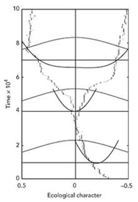
Fig 62 How a single species branches into two in the Dieckmann – Doebeli model. The three sets of curves are fitness functions. The scales are in arbitrary units used in the simulation.
The end result is identical: assortative mating can occur, opening the door to sympatric speciation.
Dieckmann and Doebeli’s mathematical model is different: it belongs to a class of models known as adaptive dynamics, and uses a differential equation rather than probabilities. That is, we write down equations that govern the rate of change of the sizes of the original population and the mutant population, and then work out the dynamics of the resulting system. Figure 62 shows a typical instance of speciation in a numerical simulation of this model.
There is also a more general way to spot the flaw in the argument that sympatric speciation is impossible: to view speciation as an example of symmetry breaking. We met this idea in the previous chapter, in connection with the markings on animals. What has symmetry breaking to do with speciation? Are species symmetric? Well ... yes. But not in the way that stripes on a tiger are symmetric.
The same mathematical concept can be realised in many different ways. The interpretation of the symmetries is very different in the applications to markings and speciation. For markings, the relevant symmetries are rigid motions; for speciation the symmetries ‘shuffle’ the organisms like a pack of cards. Only in the abstract do the two applications share the same underlying mathematics. This, in fact, is where mathematics gets much of its power: by using the same idea in different contexts.
We saw that a symmetry is a transformation that preserves structure. Here, the transformations are permutations – shufflings of labels employed in the model to identify the individual organisms. If ten identical finches are conceptually labelled 1 – 10 in some order, then the mathematical model of their interactions should not depend on the choice of labelling. All possible permutations of the numbers 1 – 10 should lead to the same model – a severe constraint on its mathematical form. On the other hand, if five finches with small beaks are labelled 1 – 5, while another five with big beaks are labelled 6 – 10, then the mathematical description should permit relabelling within each group. But it should not, for example, allow label 5 to be swapped for label 6.
From this point of view, sympatric speciation is a form of symmetry breaking. If a population of nominally identical birds evolves into two distinct groups, then the resulting system has lost some of its symmetry (such as the transformation that swaps labels 5 and 6). For several decades, mathematicians and physicists have been developing a general theory of symmetry breaking, and it is now being applied to models of speciation. One of its most striking features is that there are many ‘universal’ phenomena that do not depend on specific details of the models, only on what the symmetries are and which of them is being broken. This theory can be applied to idealised models of speciation, where it leads to at least three universal phenomena.
The first is that when a population first speciates, it usually splits into precisely two distinguishable types (Figure 63, see over). Splitting into three or more types is rare, and a mainly transitory phenomenon. The second is that the split occurs very rapidly – much faster than the usual speed of phenotypic change in the population. The third is that the two clumps will evolve in opposite directions: if one clump evolves larger beaks, then the other clump will evolve smaller beaks.
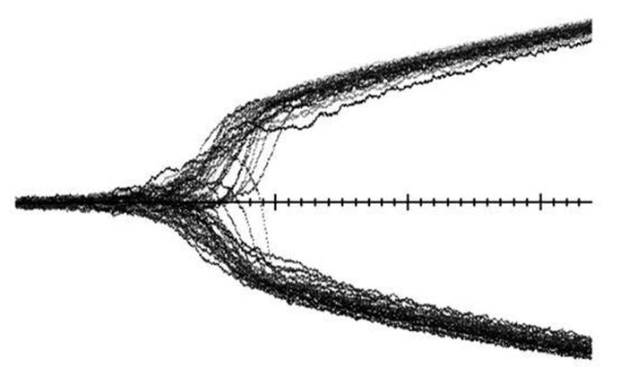
Fig 63 Simulation of sympatric speciation in a model with 50 clumps of organisms. Time runs horizontally, phenotype vertically. As time passes, a single species splits into two.
The symmetry-breaking models indicate that a key step in sympatric speciation is the onset of instability – exactly as in the game-theoretic models discussed earlier. As the environment or population size changes, the single-species state may cease to be stable, so that small, random disturbances can cause big changes. Like a stick being bent by stronger and stronger forces, something suddenly gives and the stick snaps in two. Why? Because the twopart state is stable, whereas one overstressed stick is not.
A population of organisms is stable if small changes in form or behaviour tend to be damped out; it is unstable if they grow explosively. Theory shows that gradual changes in environment or population pressure can suddenly trigger a change from a stable state to an unstable one.
There are two main forces that act on populations. Gene flow from interbreeding tends to keep them together as a single species. Natural selection, in contrast, is double-edged. Sometimes it keeps the species together, because collectively they adapt better to their environment if they all use the same strategy. But sometimes it levers them apart, because several distinct survival strategies can exploit the environment more effectively than one. In the second case, the fate of the organisms depends on which force wins. If gene flow wins, we get one species. If natural selection against a uniform strategy wins, we get two. A changing environment can change the balance of these forces, with dramatic results.
Specific mathematical models, such as those built by the Kondrashovs or Dieckmann and Doebeli, support this scenario. They provide a variety of biological mechanisms that can make the single-species state unstable and cause the symmetry to break. Intuitively, we can understand the common features of such models in simple biological terms, and suggest a genetic interpretation.
Imagine, for example, a species of finches with medium-sized beaks, all feeding on seeds from the same plant. Nominally they are all identical – that is, any differences are superficial and do not really alter the behaviour of the group. Their population expands until it is limited by the supply of those particular seeds.
Within this species, there will be a range of genetic variation, say in beak size. If the size preferred by natural selection is in the middle range, then gene flow beats environmental disruption, and the finches remain one species. The population size is well adapted to the food supply, so nothing much changes. But now suppose that a change of climate, say, reduces the food supply. Now there are advantages in having beaks that are not medium-sized, more suited to other types of seed.
A species can be thought of as a cluster in phenotypic space, so it is spread out, and not just a single point. So some birds will have slightly larger beaks than average, and others slightly smaller beaks. This is unavoidable: the average is in the middle. Birds with slightly larger beaks can feed on larger seeds. They then cease to be competition for the birds that have slightly smaller beaks. Once the balance swings in favour of avoiding the middle ground, the collective dynamics rapidly drives the birds into two distinct types. These types do not compete directly for food: instead, they avoid competition by exploiting seeds of different sizes.
As Kauffman said, once diversity has its toe in the evolutionary doorway there are many ways to amplify the split. The most obvious factor of this kind is one we have already met: assortative mating. Organisms in a given group share similar habits, eat similar food, and therefore meet up more often than they do with members of the other group. So the big puzzle is the initial split – which need not be especially large or dramatic. At a later date either of these clumps may split again, as continuing changes to the environment change the availability of resources. A cascade of such splittings leads to what biologists call ‘adaptive radiation’, where many new species arise from one ancestral species over a relatively short period.
At the moment, this kind of modelling is in its infancy. Its main contribution is to show that sympatric speciation is reasonable and natural, and to focus attention on the role of instability as a mechanism for species diversification. With more biological realism, the nature of these instabilities can be better understood.
In the meantime, the symmetry-breaking approach puts speciation in a new light. A stick breaks because the large-scale forces that act on it are inconsistent with its structural integrity. Precisely how it breaks depends on very fine detail about which fibre gives way first and how the consequences cascade – but if it didn’t happen one way, it would have to happen some other way. Whatever the details, the stick will break. Similarly, species diverge because of an unavoidable loss of stability. The actual sequence of events – which gene does what, and in what order – is less important than the context in which these events occur. An overstressed stick must break. An overstressed group of organisms must either die, or speciate.
Is there any evidence for this type of scenario? Not directly, because the timescale for the evolution of new species is too great. But there do seem to be relics of past speciation events that match the symmetry-breaking scenario very closely. A particularly informative and historically important case, which displays features consistent with various mathematical models of sympatric speciation, concerns what we now call Darwin’s finches, in the Galápagos Islands.
The Galápagos Islands form an archipelago, a group of islands, in the Pacific Ocean. They are situated at the equator, 1,000 kilometres west of the coast of Ecuador. The name comes from the Spanish word for ‘tortoise’, reflecting the presence of the celebrated giant tortoises. There were a quarter of a million of them when the islands were discovered in 1535; today they number around 15,000. The archipelago contains about ten large islands and dozens of smaller ones, all of volcanic origin.
The geology of the Galápagos Islands is unusual, and it has had a profound effect on the creatures that live there. For hundreds of millions of years the islands have followed a remarkable cycle: they rise from the ocean floor at the western edge of the archipelago, move slowly eastwards, sink beneath the waves, and eventually disappear beneath the western edge of Central America. So at any given moment, the oldest and most eroded islands are to be found in the eastern part of the archipelago, while the newest and most volcanically active are to the west.
Today we are used to the idea that continents can move, but fifty years ago it was controversial, and sixty years ago it was considered crazy. In 1912 the Berlin meteorologist Alfred Wegener took seriously a similarity that hundreds of people must have noticed: the east coast of South America and the west coast of Africa fit together like adjacent pieces of a jigsaw puzzle. He argued that this was evidence for ‘continental drift’. On geological timescales, the continents are not fixed; instead, they move, very slowly, over the surface of the planet.
The applied mathematician Harold Jeffreys objected that no physical mechanism can exert the gigantic forces required to make continents plough through the ocean floor. This was entirely correct; nevertheless, by the 1960s it became clear that Wegener was right. The ocean floor moves along with the continents, like a giant conveyor belt. New floor forms along mid-ocean ridges as magma wells up from the Earth’s mantle, cools and spreads sideways; old floor is ‘subducted’, sliding back down into the mantle at the edges of continents. Indeed, it is sometimes pulled down. As a result, the surface of the Earth is divided into eight major ‘tectonic plates’ and many smaller ones. These plates are effectively rigid, yet they can move in complex ways, driven by huge convection currents in the molten rock of the Earth’s mantle. They interact along their common boundaries.
The Galápagos Islands are poised at the junction of three plates: the Cocos, Nazca and Pacific plates. This meeting point, known as the Galápagos Triple Junction, is geologically unusual because the plates do not meet in a simple Y shape. Instead, two much smaller ‘microplates’ seem to be trapped at the junction, and they spin in synchrony with each other like two adjacent gearwheels. The Canadian geologist J. Tuzo Wilson explained this curious behaviour in 1963, suggesting that beneath the islands there is a geological ‘hot spot’ where a huge plume of molten magma rises up through the mantle, breaks through the ocean crust and forms volcanic cones. A similar hot spot is thought to create the Hawaiian island chain, but those do not lie on a plate boundary. For at least 20 million years, the Galápagos hot spot has remained in much the same place, though it has wobbled a little; the ocean floor has drifted eastward across it, carried by the movement of the tectonic plates. Currently the Nazca plate is moving at a speed of 60 kilometres every million years, while the Cocos plate moves 80 kilometres every million years. These speeds might seem too small to matter, but continental drift would carry a Galápagos island to the mainland of South America in a mere 12 million years, very short by geological standards.
The Hawaiian islands seem to have formed one at a time, each volcano becoming dormant as it is carried away from the hot spot, but the Galápagos Islands are more complicated. Nearly all of them have been volcanically active in the last few hundred years, which geologically is a mere instant, and their periods of formation have overlapped substantially. Today the newest island in the archipelago is Fernandina, which is an active volcano.
As a consequence of their isolation and continual tectonic turnover, the Galápagos Islands are a bit like the well-known axe, the exact same axe that my father gave me, though it has had three new heads and four new handles. This rapid turnover of land has made the flora and fauna of the Galápagos unlike any elsewhere on the planet. Darwin spent five weeks in the Galápagos. Walking over jagged fields of coal-black lava, he was struck by the realisation that this was new land, and that its outlandish creatures must be new arrivals. Much later, what he found there started to sink in, and it had a big effect on him. None of this (aside from a few general remarks from the second edition onwards) appears in the Origin, but his letters and notebooks show how important the Galápagos Islands were to his thinking.
Darwin was an obsessive collector, and he brought back a collection of dead birds from the Galápagos. He thought they were varieties of blackbirds, finches and ‘gross-beaks’. The ornithologist John Gould looked at the specimens and told Darwin that they were all finches – a dozen or so distinct species. They differed in body size, in colouring and, especially, in the shapes and sizes of their beaks. The differences were not huge, but enough to indicate distinct species. Today they are known collectively as Darwin’s finches, a name dating from 1936, and we recognise 13 species in the Galápagos10 plus another on the Cocos Islands.
In The Voyage of the Beagle, based on his diary, Darwin wrote:
The remaining land-birds form a most singular group of finches, related to each other in the structure of their beaks, short tails, form of body, and plumage: there are thirteen species, which Mr. Gould has divided into four sub-groups. All these species are peculiar to this archipelago; and so is the whole group, with the exception of one species ... The males of all, or certainly of the greater number, are jet black; and the females (with perhaps one or two exceptions) are brown. The most curious fact is the perfect gradation in the size of the beaks in the different species of Geospiza, from one as large as that of a hawfinch to that of a chaffinch, and ... even to that of a warbler ... Seeing this gradation and diversity of structure in one small, intimately related group of birds, one might really fancy that from an original paucity of birds in this archipelago, one species had been taken and modified for different ends.
Because Darwin uncharacteristically omitted to record on which island he collected which specimen, he missed a smoking gun for natural selection: the finch species are often different on different islands. But we now know that Darwin’s intuition was correct. The closely related genetics of Darwin’s finches show that they diverged from a single ancestral group about five million years ago. (Perhaps a few founders were blown to the islands from the Central American mainland by a storm, but that’s conjectural.)
The first systematic study of the genetics and behaviour of Darwin’s finches was made by David Lack. Working as a schoolmaster in Devon and later as field ornithologist at Oxford, he wrote two books with the title Darwin’s Finches: a scholarly one in 1945, and a more popular account in 1961.11 Lack visited the Galápagos in 1938, and among other things, he measured the sizes of various birds’ beaks. In his first book he suggested that the differences in size were recognition signals – birds could distinguish their own species by looking at the beaks. So he viewed beak sizes as an isolating mechanism, something that prevented gene flow even when it would otherwise be possible. But by 1961 Lack had revised his opinion, and now saw the differences in size as evolutionary adaptations to different food sources. Later studies confirm that view.
Lack’s work has been continued by Peter and Rosemary Grant, husband and wife, both emeritus professors at Princeton. Since 1973 they have spent half of every year on the tiny Galápagos island of Daphne Major, capturing and releasing the birds, tagging them, measuring their sizes and shapes, and taking blood samples. Through their efforts we now know a great deal about Darwin’s finches, their behaviour, form and genetics.
One of the main implications of the symmetry-breaking model of sympatric speciation is striking: the two new phenotypes move away from the old one in opposite directions.12 If, for example, a finch species with medium-sized beaks splits into two distinct species distinguished by beak size, then one will have bigger beaks and the other smaller beaks.
No such splitting has been observed directly, but that is to be expected because the evolutionary timescale is so long. Instead, we might hope to find modern traces of the evolutionary process. Fossil Darwin’s finches would be lovely, but the Galápagos Islands are volcanic, and fossils hardly ever form in volcanic strata. However, there is another type of ‘fossil’ – the modern species themselves. These display a phenomenon known as character displacement: the phenotypes of distinct species change if both those species are present in a given environment. With a bit of imagination, you can view these changes as a kind of modern reconstruction of the likely evolution of the two species.
The species concerned are the medium ground finch Geospiza fortis and the small ground finch G. fuliginosa, henceforth Medium and Small. The character concerned is beak depth, the width of the beak at its base. Medium is found on the island of Los Hermanos (Crossman), but Small is not. Conversely, Small is found on Daphne, but Medium is not. However, both species coexist on Isabela (Albemarle).
When only one species is present, the beak depth is the same for either of them: the mean beak depth for Medium is very close to 10 mm on Los Hermanos, and the same holds for Small on Daphne. But when they coexist, they force each other apart: the mean beak depth for Medium on Isabela is very close to 12 mm, but that for Small is 8 mm. The average of 8 and 12 is 10: neatly consistent with the prediction made by the symmetry-breaking model of sympatric speciation. It is also worth noting that the other kinds of model used by the Kondrashovs and by Dieckmann and Doebeli also possess this ‘constant mean’ property.
This is character displacement, not speciation as such. But it can be argued that when the two species are placed in the same environment, we are reconstructing the original evolutionary competition ... and finding out what the result was. I don’t claim that this observation is anything more significant than a straw in the wind, and grasping at straws is not always to be recommended. But it’s intriguing to encounter exactly the predicted behaviour in the most famous example of speciation that there is – and the one that Darwin nearly missed.