Mathematics of Life (2011)

Chapter 15. Networking Opportunities

As we’ve seen when looking at the brain in Chapter 11, networks are hot property in biology and mathematics. They are hot property in physics and engineering too, and a popular buzzword in the business world. If you work in science or in commerce, it is very difficult not to run into networks. A ubiquitous example is the Internet, which by definition is a network of intercommunicating computers.

Networks abound in biology. We’ve already seen how the ability of nerve cells to network allows relatively simple components to produce rich and subtle types of behaviour. Indeed, if the ‘connectionist’ view of the human mind is anywhere near the truth, our ability to behave intelligently, our conscious awareness and our feeling (rightly or wrongly) that we have free will are all consequences of two things: the brain’s intricate network of neurons, and its interactions with the body that contains it and with the external world.

In the case of the human nervous system, the network is a physical thing. Nerve cells are linked together by axons and dendrites, the body’s hidden wiring. In most biological networks this linkage is more metaphorical. Ecologists study food webs in an ecosystem: which organisms feed on which. A food web is a network in which real organisms are ‘linked’ conceptually by the relationship of eating one another. Disease transmission can be thought of as a network in which individual people are linked by infection. A species can be thought of as a network of organisms, linked by everyday interactions such as competition for food or mates, and social behaviour.

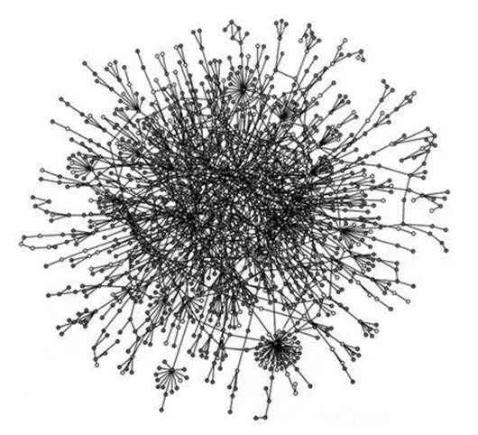
Fig 64 Network of protein interactions in yeast.

Some of the most important but least understood networks arise at the molecular level. We now know that biological development, in which a fertilised egg turns into an organism, is not just a matter of reading off information from DNA. Some parts of the genome, genes in the strict sense, provide instructions for making proteins. More precisely, they encode the order in which the constituent amino acids must be assembled: DNA doesn’t perform the assembly. However, an organism is not just a bag of proteins: the right protein has to end up in the right place, and the entire system has to function as a living creature. One way to get protein to the right place is to make it there, and this involves switching the activity of a gene on or off depending on which cell it is in and where that cell is currently located in the organism. This switching is itself controlled, in part, by other genes, whose activity may be regulated by yet other genes. Collections of genes combine together to form genetic regulatory networks, and our understanding of how DNA affects development, and the day-to-day running of the body for that matter, depends on sorting out what these regulatory networks do and how they do it (see Figure 64).

Social networking has become fashionable among humans, thanks to sites such as Facebook and Twitter. A real network, the Internet, helps us set up and maintain these social connections, but the social network is metaphorical. We were anticipated, millions of years ago, by an organism whose natural social behaviour sometimes creates real networks.

You wouldn’t sign a contract with Physarum polycephalum for designing a railway system. For a start, it can’t read or write: it is a species of slime mould. Its name means ‘many-headed slime’, and that’s what it’s often called. It can’t compete in the intelligence stakes with humans, dolphins, octopuses or even mantis shrimp. There is dumb, there is dumber ... and there is slime mould.

However, this slime mould can indeed design railway systems. It does need a bit of prompting, but it does a pretty good job. In fact, as Atsushi Tero at Hokkaido University in Japan and a team of eight other researchers discovered early in 2010, P. polycephalum comes up with almost the same design for the Tokyo rail system that the engineers did.¹ And all they ‘told’ the slime mould was where the main cities are; the mould did the rest.

A few other scientists have persuaded slime moulds to solve other kinds of networking problems, such as finding their way through mazes. In principle, you could build a slime mould computer and do word processing on it, though it might take half the age of the universe to get as far as the first sentence. The slime mould’s talents are not really suited to processing digital information at high speed. But when it comes to networks, slime mould is in its element.

Using slime mould to design a railway system is not as crazy as it sounds, because there are environmental conditions that cause slime moulds to structure their colony into a network of vein-like tubes, and to transport vital fluids along those tubes. A train system transports people along railway lines – it’s actually a very similar problem. As well as using the slime mould to solve a problem about networks, the Japanese team used the mathematics of networks to find out how the slime mould did it, neatly closing the conceptual circle. The result might even be useful for human designers; not by using the slime mould to solve real design problems, but to simulate its strategies on a powerful computer.

P. polycephalum is a single-celled organism, a bit like an amoeba, except that this cell contains a large number of nuclei. Like an amoeba it can extend protuberances, which it uses to explore its surroundings – in effect, to go hunting for food. It spreads over dead logs or rotting leaves in a slimy yellow carpet, and the hunting goes on along the edge of the carpet, where individual ‘plasmodia’, regions that contain a single nucleus, seek food. Inside this exploratory boundary the organism forms itself into a network of tubes, reminiscent of the veins on the back of the human hand; just like veins, these tubes carry fluid, but the fluid is the protoplasm that makes up the interior of the cell. The protoplasm carries particles of food and other vital molecules as it flows, distributing the bounty to the entire organism.

Bizarre as this lifestyle may seem, it’s an effective way to make a living, and slime moulds are very common. If you want to harness the networking abilities of slime mould, you have to present your computation to them in a form that appeals. And what appeals to a slime mould is food.

In its experiments, the Japanese team placed food sources on a flat surface at locations corresponding to the 36 main cities in the region. Think of it as a map of the area around Tokyo, with blobs of food for cities, but with no connecting roads or railways marked, because those would prejudice the procedure. Then they set their slime mould loose, by introducing a plasmodium at Tokyo and allowing it to go hunting.

To begin with, the plasmodium didn’t have a clue where the food was, so it spread all over the map, forming a flattish layer. But as time passed, the layer contracted to form a network of tubes, linking the food sources. To avoid biasing the results by starting from Tokyo, the researchers performed another experiment, but this time they started with the mould spread all over the map. The results were very similar. To make sure that the mould formed a network, rather than just remaining spread out, they allowed any excess to spill over onto a large food source outside the area of the map.

The resulting network was very like the actual rail network connecting these cities (Figure 65, see over). The resemblance got better when the slime mould was deterred from entering what in the real world were mountainous regions by a light being shone on the corresponding bits of the map (P. polycephalum tends to avoid light). In effect, the researchers used light intensity to simulate terrain. With or without this extra tweak, the slime’s network and the real one performed very similarly, according to a number of different measures of efficiency, such as the ratio of benefits to costs.

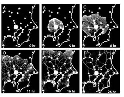
Fig 65 How the slime mould built its railway: six stages in the evolution of a biological network.

This behaviour is not entirely surprising, but there is a sign that something interesting is going on. The slime mould does not simply ‘triangulate’ the entire region by forming tubes between all neighbouring cities. Neither does the rail network. Both leave out potential links – and both leave out much the same links.

Is this similarity between the two networks a superficial accident, or a sign of shared origins? It’s a bit of both. It might seem that the Tokyo network was ‘designed’, while the slime mould one evolved. Engineers worked out where to run the railway lines; the slime mould modified its network by expanding some tubes and contracting or eliminating others. But the real rail network also evolved: as cities appeared and grew, the rail system grew with it, adding new links. As the numbers of passengers increased, more lines and more trains were constructed, ‘strengthening’ the links in the network. Services that did not attract customers were abandoned.

If the engineers had been starting from scratch, with all cities in place but no rail network, they could have adopted a more rational and more global approach, designing the entire network to optimise whatever quantities seemed appropriate, such as transporting the required number of people cheaply and quickly. The slime mould could not have taken this approach. However, the engineers might still learn some useful tricks from the slime mould, as the Japanese team discovered when they devised a mathematical model of what the slime mould was actually doing.

Their model starts with a very fine random mesh of thin tubes, resembling the initial layer where the slime mould spreads all over the map. They wrote down simple equations for the amount of fluid that could be pumped through each tube, based on standard ideas from fluid dynamics. Their equations state that the amount of fluid flowing through a tube is proportional to the difference in pressure between its two ends, to its ‘conductivity’ (a measure of how big the tube is, proportional to the fourth power of its radius) and inversely proportional to the length.

To modify the sizes of the tubes, choose two random cities. Pump in extra fluid at one of them and extract it at the other, so that the total amount of fluid stays unchanged. Calculate the amount of fluid passing along each tube, using the equations. Make small changes in the diameters of the tubes, so that the ones carrying large amounts of fluid get bigger, and the ones carrying small amounts of fluid get smaller. Work out whether the change improves the efficiency of the network. If so, keep it; if not, try another random change. The exact method for doing this allows tubes to contract completely, attaining zero diameter: when that happens, they disappear from the network. Repeat this procedure over and over again, with new random choices of the two cities, and keep going until the structure settles down to something that hardly changes from one stage to the next.

Efficiency can be measured in many different ways: how much material can be transported, how rapidly it can be transported, how much benefit is gained for given cost. This evolutionary process can be deliberately tweaked to enhance any desired measure of efficiency: it is just a matter of selecting appropriate rules for how fast the tubes change in response to the quantity of fluid they are transporting. The team found that one tweak of this kind led to a network that in some ways outperformed both slime mould and the actual Tokyo rail system: it had the same transport efficiency but a better benefit-to-cost ratio. However, this network was more fragile: its ability to transport fluid (or people) declined significantly if parts of it were damaged or removed, whereas the slime mould network and the rail system are more robust.

There are other mathematical techniques for linking cities in a network, and the team compared their results with these as well. In cost terms alone, the most efficient network is a ‘Steiner spanning tree’, which has branches but no closed loops; in such an arrangement, whenever a branch splits at a Y-shaped junction, the angles in the Y are all 120°. This is the network that uses the shortest length of rail. But it is not a terribly good way to transport people, or slime mould protoplasm, because the link between two nodes can go all round the houses – from a distant city into the centre of Tokyo and out again, for instance. So travel time can be unnecessarily large. Neither the rail network nor the slime mould one looks remotely like a Steiner spanning tree.

Tero and his colleagues sum up their results like this:

Our biologically inspired mathematical model can capture the basic dynamics of network adaptability through iteration of local rules and produces solutions with properties comparable to or better than those of real-world infrastructure networks. Furthermore, the model has a number of tunable parameters that allow adjustment of the benefit/cost ratio to increase specific features, such as fault tolerance or transport efficiency, while keeping costs low. Such a model may provide a useful starting point to improve routing protocols and topology control for self-organized networks such as remote sensor arrays, mobile ad hoc networks, or wireless mesh networks.

Networks entered mathematics through a puzzle. In 1735 the prolific Leonhard Euler turned his mind to a topic of conversation among the good folk of Königsberg, then a city in Prussia, now Kaliningrad in Russia. The city was located on both banks of the River Pregel, and boasted seven bridges. These linked two islands to the banks, and to each other (see Figure 66). The burning issue was this: is it possible to take a walk that crosses each bridge exactly once?

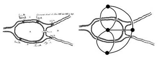
Fig 66 Problem of the Künigsberg bridges. Left: Euler’s original puzzle. Right: Turning the puzzle into a network.

Euler didn’t find a solution. He did something more difficult – he proved that no solution exists. His insight was to strip the problem down to its essentials. All that matters is how the land masses are connected. Their size and shape are irrelevant; worse, they get in the way of thinking about the problem. His actual argument was algebraic, assigning symbols to the land masses and the bridges, but soon afterwards it was reinterpreted graphically, a much more vivid way to represent the problem. This reduces the puzzle to a diagram in which dots are joined by lines, which I’ve superimposed on the map on the right of Figure 66.

In this diagram, each land mass – north bank, south bank and the two islands – corresponds to a dot, and we join two dots by a line whenever a bridge links the corresponding land masses. Altogether, we get four dots and seven lines. The puzzle now translates into a simple question: is there a path that includes each line exactly once? Euler discussed open paths, which start and end at different dots, and closed paths, which start and end in the same place. He proved that neither kind of path exists for the Königsberg bridge diagram. More generally, he characterised diagrams for which such paths do or do not exist.²

This kind of diagram was originally called a ‘graph’, but nowadays an increasingly common alternative is the more evocative and less ambiguous network. Euler’s simple theorem about a puzzle was the first evidence for a broad principle: the architecture (or topology) of a network has a huge influence on what it can do.

Mathematically, a network consists of nodes (dots, vertices) linked together by edges (lines, links, connections, arrows). The nodes represent some kind of component, or agent, and two nodes are joined by an edge if and only if they interact. Edges may be bidirectional (interactions go both ways) or unidirectional (A influences B but not the other way round). The unidirectional case yields a directed network, whose edges are usually drawn as arrows. The edges may carry ‘weights’ to indicate the strength of the interaction. They may be of different kinds (fox predating on rabbit is different from rabbit predating on vegetation) or they may be nominally identical (fox A predating on rabbit X is near enough the same as fox B predating on rabbit Y).

Two graphs have the same architecture (or topology) if one graph can be obtained by rearranging the positions of the other one’s nodes and edges, while maintaining the same connections and arrow directions (and any additional decoration such as weights or types of edge). Important architectures include chains, rings, complete graphs and random graphs, as shown in Figure 67.

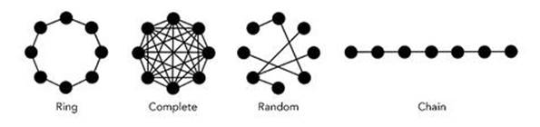
Fig 67 Four types of network. Here all edges are bidirectional.

We can investigate networks in the abstract, in concrete mathematical models where the nodes and edges have additional structure, and in real networks with real agents and interactions. These three contexts are closely associated, but it is important to bear in mind that they are different. As long as we do that, we can safely employ the same words in all contexts – for example, talking of a rabbit as a node in a food web and drawing it as a dot.

Different people use networks for different purposes and ask different questions. An early pioneer was Stuart Kauffman, who employed binary switching circuits (each node can be either on or off) to model gene interactions in a cell. He found that the dynamics of the network depended critically on the average number of edges linked to each node. Innumerable types of network have been studied: discrete (cellular automata), continuous (differential equations), probabilistic (Markov chains), fractal (iterated function schemes). Many complex systems are networks. A radically new network architecture that has attracted attention is the small world: a regular network with near-neighbour connections, in which some edges are randomly rewired to become long-range connections, or some nodes become ‘hubs’ that are connected to unusually many other nodes.

There are several general theories of network structure and behaviour. Intensive work on statistical properties of random networks shows that as the probability of including any given edge increases, there is a transition at which most of the nodes suddenly link up into a single giant component. This result, metaphorically at least, has an application to epidemics. Here the nodes are people and edges indicate infection. The existence of a giant component shows that if the probability of disease transmission becomes sufficiently great, almost everyone will be exposed. Less obviously, it implies that there is a sharp threshold, below which the infection remains in numerous small ‘pools’ isolated from one another, and above which nearly everyone is exposed.

Another approach, introduced by the Japanese physicist Yoshiki Kuramoto, analyses network dynamics in which the effect of each node on those to which it is linked is small.³ Think of an epidemic that is rarely infectious, for example. With these assumptions, useful quantitative predictions can be made about the behaviour of the network and its stability. More recently, theories have been devised to incorporate stronger connections and more exotic behaviour, including dynamical chaos.

In 1996 Joanne Collier, Nicholas Monk, Philip Maini and Julian Lewis, a group of mathematical biologists at Oxford University, used a mathematical model to investigate a mysterious patterning process that had been observed in insects, nematode worms, chickens and frogs.⁴ Cells can differentiate under the influence of suitable control genes and signals; that is, cells that originally have the potential to change into several different cell types choose one type and change into that. It is as if the genetic signals determine the cell’s fate, and indeed this is the term that biologists often use. In some developing tissues, a mass of identical cells somehow differentiates into many types. Some apparently random collection of cells ends up with one fate, while the cells next to them have a different fate. The resulting cell types (there may be more than two) are intimately mixed.

The mechanism behind this process appears to have evolved early on, and is highly conserved: despite the effects of natural selection, it has not greatly changed over many hundreds of millions of years. This implies that it must have had been so biologically significant that any mutations in the associated DNA code were weeded out, so it is actually conserved because of natural selection.

At first sight this intimate mixture of fates seems puzzling, but there is a relatively easy way to achieve it: instruct each cell ‘Be different from your neighbours’. This mechanism is known as lateral inhibition. An example is the nervous system. Since nerve cells form networks with long thin connections, and their ability to function depends on this geometry, it’s not a good idea for the near neighbours of nerve cells to also become nerve cells. Experiments support the notion that when a cell develops into a nerve cell, it sends signals to nearby cells telling them not to do the same.

You can sometimes spot the genes responsible: if they experience a mutation, the process goes wrong and the mixed pattern fails to develop. Such observations have been recorded in the geneticists’ favourite organism, the fruit fly Drosophila. But even if the gene responsible for lateral inhibition is known, one further puzzle remains: which cell initiates the process. In order to inhibit a neighbour, a cell must already be actively differentiating. Is the starting point also determined by some gene, or can lateral inhibition alone produce the required mixture of cell types? This is the problem that the four mathematical biologists tackled.

Experiments show that the main gene responsible for lateral inhibition is one known as Notch, and it acts in concert with another gene, Delta, that triggers the formation of neurons. Both of them generate molecular signals, in the form of proteins, that can pass from cell to cell. So the mathematical model needs to take account of these genes and how they interact and are transmitted from cell to cell. The researchers looked at two spatial arrangements of cells: a line of adjacent cells, and a plane covered in a hexagonal array, like a honeycomb (see Figure 68). Both arrangements are idealised compared with real tissues, but they capture the main features of the system in a simple way. Both are networks: place a dot at each cell and draw edges from that cell to its immediate neighbours.

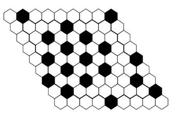
Fig 68 Pattern of primary-fate cells (black: high Notch activity) and secondary-fate cells (white: low Notch activity) in a hexagonal lattice.

The team set up suitable equations and used a computer to solve them numerically. The results confirmed that if there is strong enough feedback in the system, then initial tiny differences between neighbouring cells will automatically be amplified. In fact, this is another instance of symmetry breaking, analogous to the way slight variations in the height of a flat desert are amplified by the wind to create huge dunes. Here, the pattern is one of gene activity: cells with high levels of Delta activity and low levels of Notch activation are scattered among cells with low Delta activity levels and high Notch activation levels. These represent the two distinct fates of the original homogeneous array of cells.

The simulations often led to irregular patterns, but in every case the irregularities took the form of two adjacent cells with high levels of Notch activity. Two neighbouring cells with low levels of Notch activity never occurred. Experiments show the same effect: lateral inhibition causes primary-fate cells to be separated by at least one secondary-fate cell, but secondary-fate cells may be adjacent to one another.

The main conclusion answers the question raised earlier: it is not necessary to specify the cell that initiates the pattern. Instead, random fluctuations will amplify some initial tiny difference, producing large-scale patterns. Similarly, a desert does not have to be told which grain of sand will trigger dune formation.