Mathematics of Life (2011)
Chapter 16. The Paradox of the Plankton
The uppermost layers of Earth’s oceans teem with plankton, organisms ranging from microscopic creatures to small jellyfish. Many are the larvae of much larger adults. They all occupy the same kind of habitat and compete for much the same resources, which is why they are all classed together under a single catch-all name. However, there is a long-standing biological principle, introduced in 1932 by the Russian biologist Georgyi Gause: the principle of competitive exclusion. This states that the number of species in any environment should be no more than the number of available ‘niches’ – ways to make a living. The reasoning is that if two species compete for the same niche, then natural selection implies that one of them will win.
This is the paradox of the plankton: the niches are few, yet the diversity is enormous.
The paradox is a problem in ecology: the study of systems of coexisting organisms. Although it is often convenient for biologists to study a given organism in isolation, as if nothing else existed, the real world isn’t like that. Organisms are surrounded by, and often inhabited by, other organisms. The human body contains more bacteria – useful bacteria, vital to such functions as digesting food – than it does human cells. Rabbits coexist with foxes, owls and plants. These creatures interact with one another, often strongly: rabbits eat plants, while foxes and owls eat rabbits. Indirect interactions also occur: owls don’t eat foxes (except perhaps very young ones), but they do eat the rabbits that the fox is hoping will make the next meal. So the presence of owls has an indirect effect on the fox population.
In 1930 the British botanist Roy Clapham recognised the interrelated nature of living creatures by coining the word ‘ecosystem’. This refers to any relatively well-defined environment, plus the creatures that inhabit it. A woodland and a coral reef are both ecosystems. In a sense, the entire planet is an ecosystem: this is the essence of James Lovelock’s famous Gaia hypothesis, often stated as ‘the planet is an organism’. In recent years it has been recognised that if we are to ensure the continued health of the global ecosystem, and of its important subsystems, we need to understand how ecosystems work. What makes them stable, and what factors create or destroy diversity? How can we exploit the oceans without making many species of fish extinct? What effect do pesticides and herbicides have, not just on their targets, but on everything around them? And so a new branch of science was born: ecology, the study of ecosystems.
An apparently different, but closely related, branch of biology is epidemiology, the study of diseases. The subject can be traced back to Hippocrates, who noticed that there was some kind of connection between disease and environment. He introduced the terms ‘endemic’ and ‘epidemic’, to distinguish diseases that circulated within a population from those that came from outside. Modern examples in the UK are chickenpox and influenza, respectively. Epidemiology is similar to ecology because it also deals with populations of organisms within an environment. However, the organisms are now microorganisms such as viruses and bacteria, and the environment is often the human body. The two subjects start to overlap when transmission from one person to another comes into play, because now we have to consider populations of people as well as populations of disease organisms. It is, then, no great surprise to find that similar mathematical models arise in both subjects, which is one reason to treat them as variations on the same overall theme.
A basic problem in both areas is to understand how populations of organisms change over time. In many parts of the world we find boom-and-bust cycles, where a population of, say, gannets grows rapidly, exceeds the available food supply, and crashes, then repeats the same process. The resulting ‘cycle’ need not repeat exactly the same numbers, but it repeats the same sequence of events. This corner of ecology is known as population dynamics.
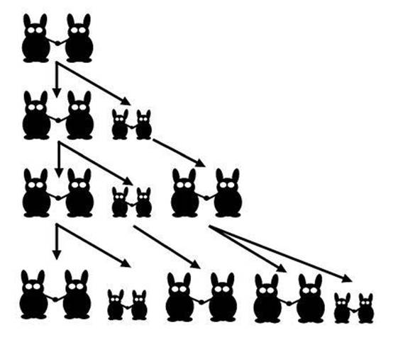
Fig 69 The first few generations in Fibonacci’s rabbit model.
The earliest mathematical model of the growth of a population seems to be Leonardo of Pisa’s famous rabbit problem of 1202, mentioned in Chapter 4 in connection with plant numerology. Start with one pair of immature rabbits. After one season, each immature pair becomes mature, and each mature pair gives rise to one immature pair (see Figure 69). If no rabbits die, how does the population grow? Leonardo, usually known by his nickname Fibonacci (son of Bonaccio), showed that the number of pairs follow the pattern
![]()
in which each number after the first two is the sum of the two that precede it. As we saw, these are called Fibonacci numbers. They have many interesting features; for example, the nth Fibonacci number is very close to 0.724×(1.618)n.1 So Fibonacci’s little puzzle predicts exponential growth: as we go further and further along the sequence, we find that each successive number is (very close to) the previous one multiplied by a constant amount, here 1.618.
The model is of course not realistic, and was not intended to be. It assumes that rabbits are immortal, that the rules for the birth of new rabbits are universally obeyed, and so on. Fibonacci didn’t intend it to tell us anything about rabbits: it was just a cute numerical problem in his arithmetic textbook. However, modern generalisations, known as Leslie models, are more realistic: they include mortality and age structure, and have practical applications to real populations. More about these models shortly.
For large populations, it is common to employ a smoothed or continuum model, in which the population is represented as a proportion of some notional maximum population, which means that it can be thought of as a real number. For example, if the maximum population is 1,000,000 and the actual number of animals is 633,241, then the proportion is 0.633241, and the discrete nature of the population is visible only in the seventh decimal place. That is, all digits from that point on are zero, whereas in a true continuum they could take any values.
One of the simplest such models of the growth of a species of organism is the logistic equation.2 It states in mathematical formulas that the growth rate of the population is proportional to the number of animals, subject to a cut-off as that number approaches the carrying capacity of the environment – a notional upper limit to the size of a sustainable population. The solution is known as a logistic or sigmoidal (S-shaped) curve, and it can be described by an explicit mathematical formula. The population starts near zero. At first it increases almost exponentially, but then the growth rate starts to level off. The rate of increase of the population reaches its highest value, and then starts to decrease. Eventually the size of the population levels off at a value that gets ever closer to, but never quite reaches, the carrying capacity. The maximum growth rate occurs when the population is precisely half the carrying capacity.
If a population of animals obeys the logistic equation, you can observe when the growth rate peaks, and that enables you to predict that its final size will be twice as big. Figure 70 is a classic example, from Gause’s The Struggle for Existence, showing growth curves for two yeast species, Saccharomyces and Schizosaccharomyces, derived from 111 experiments. It also shows the pattern of growth when the two species coexist.
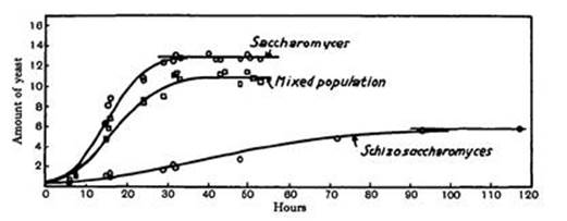
Fig 70 Gause’s observations of the growth of yeast.
The logistic growth pattern is not realistic in many circumstances, and many other models of population growth have been devised. The principles underlying these models are relatively simple: at any given instant the total population in the immediate future must be the population now, plus the number of births, minus the number of deaths.
Leslie models, the more realistic generalisations of Fibonacci’s rabbits, provide a simple example of how these principles can be implemented. They are named after Patrick Leslie, an animal ecologist who developed them in the late 1940s. They are based on a table of numbers called the Leslie matrix. A simple example captures the basic ideas, and practical models are more elaborate versions of the same thing.
Suppose we modify Fibonacci’s set-up to allow three age classes of (pairs of) rabbit: immature, adult and elderly. We let time tick by in discrete steps, 1, 2, 3, and so on, and assume that at each step immature pairs become adult, adults become elderly and elderly ones die. Additionally, each adult pair gives birth, on average, to some number of immature pairs (which may be a fraction because we’re working with the average). Call this the birth rate, and assume for the sake of illustration that this is 0.5. Immature pairs and elderly ones have no offspring.
The state of the population at any given time-step is given by three numbers: how many immature, adult and elderly pairs there are. Moreover, at the next time-step:
• The number of immature pairs is equal to the previous number of adult pairs multiplied by the birth rate.
• The number of adults is equal to the previous number of immature pairs.
• The number of elderly pairs is equal to the previous number of adult pairs.
These rules can be turned into a table of numbers, which in this case looks like this:
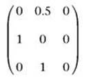
This is called a Leslie matrix, and shows how the three age classes included in the model change at each time-step. In order from left to right and top to bottom, the age classes are immature, adult, elderly. The entry in a given row and column tells us what proportion of pairs in that column become, or give birth to, a pair whose age class corresponds to the chosen row. For example, the top row (0, 0.5, 0) says that we get 0 immature pairs from each immature pair, 0.5 immature pairs from each adult pair and 0 immature pairs from each elderly pair.
The Leslie matrix encodes the rules for all transitions among age classes, which can be more complicated than the ones I chose. There might, for instance, be ten age classes, and most of those might have various non-zero birth rates. The top row would then become a longer sequence of specific, usually different, numbers. A formula that incorporates this matrix can then be used to calculate how the numbers of pairs in the three age classes change over time.
A theoretical analysis of this formula reveals that for any model of this kind, there is a unique ‘steady’ age structure and overall growth rate, and that almost any initial choice of numbers for the various age classes ends up looking like this steady state.
For my choice of matrix, the steady age structure is approximately 23% immature, 32% adult and 45% elderly. The total population drops by 29% at each time-step (which reflects the low birth rate of 0.5, below replacement level). So this population of rabbits will eventually die out, rather than exploding like Fibonacci’s rabbits.
If instead the birth rate were 1, the population would approach a fixed size; if the birth rate were larger than 1, the population would explode. This tidy transition at birth rate 1 arises because only adults have offspring. With more age classes there are several birth rates, and the change from dying out to exploding is more complicated.
An important application of such models is the growth of the human population, currently estimated to be just under 7 billion. Very sophisticated models are needed to predict future growth, because this depends on age distribution, social changes, immigration, and many other social and political features. But all models must obey the basic ‘law of conservation of people’: people can be created by birth, they can be destroyed by death and they can move from one nation to another, but they can’t (astronauts excepted) vanish into thin air.
This law can easily be turned into mathematical equations, but the form of the equations depends on the birth rate and the death rate, and on how these change as the population itself changes. Leslie models use constant birth rates for each age class, and split the population into a fixed number of age classes. Other models replace these assumptions by more realistic ones: for instance, the birth rates might depend on the overall population size, or people might remain in a given age class for a certain time before moving to the next one.
A good model requires realistic formulas for all birth and death rates. These can be obtained if good data are available, but for the world population accurate data exist only from 1950 to the present. This is too short a time span to determine, with any certainty, the specific form that the equations should take. So experts make informed guesses and choose what seems most reasonable. Not surprisingly, different experts prefer different models. Some use deterministic models, some use statistical ones. Some combine the two. Some are orthodox, some not.
In consequence, there is a lot of disagreement about when the Earth’s population will peak, and how big it will be when it does. Predictions range from 7.5 billion to 14 billion. Figure 71 shows the growth since 1750, with a short prediction in the middle of that range. The evidence suggests that the rate of growth has been fairly constant since the 1970s, when the population reached 4 billion, so there is no clear evidence that the growth rate is slowing down, let alone that it will level off or start to decline. Nonetheless, the world population is generally expected to peak some time in the next 150 years. The main reasons for this expectation are social and cultural. An important one is the ‘demographic transition’, in which improved education and standard of living cause a sharp fall in the size of families. But in many countries this is offset by rising life expectancy, caused by improvements in medicine and standard of living.
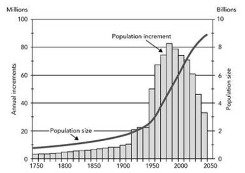
Fig 71 Long-term world population growth, 1750 – 2050 (predicted after 2010.) The curve shows population size, bars show increases in size at intervals of 2.5 years.
It is difficult to incorporate these effects into population models, because they depend on scientific advances, political changes, and cultural shifts, all of which are inherently unpredictable. Statistical methods are often used, and like all statistics they work better for large populations. So, just as it turns out to be easier to forecast the global climate than to predict local weather, it is easier to forecast the general trend of the global population than it is to predict national populations. But even then, the uncertainties are huge.
The traditional states seen in dynamical systems are steady states (also called equilibria), where nothing changes as time passes, and periodic states, where the same sequence of events repeats over and over again. A rock is in a steady state if it’s not moving and we ignore erosion. The cycle of the seasons is periodic, with period one year. But in the 1960s mathematicians realised that tradition had completely missed another, more puzzling kind of behaviour: chaos. This is behaviour so irregular that it may appear random, but it arises in models without explicit random features, for which the present completely determines the future. Such models include all dynamical systems.
At first, many scientists viewed chaos with suspicion, presumably because they thought that such outlandish behaviour had no place in nature. But chaos is entirely natural: it arises whenever the dynamics of a system mixes it up, much like kneading dough mixes the ingredients. One consequence is the ‘butterfly effect’, which originally arose in weather forecasting. In principle, and in a very specific sense, the flap of a butterfly’s wing can change the global weather pattern. More prosaically, although the future of the system is completely determined by its present, this requires knowing the present to infinite accuracy. In practice, tiny measurement errors in determining the present state grow rapidly, making the future unpredictable beyond some ‘prediction horizon’.
As soon as mathematicians started to think about dynamics geometrically, chaos became obvious. It only seems outlandish if you are looking for solutions that can be expressed by neat, tidy formulas. And those are rare.
In fact, it was geometric thinking – about the stability of the Solar System – that led the French mathematician Henri Poincaré to discover chaos in 1895. A few sporadic developments occurred during the first half of the twentieth century, but it all came together in the 1960s when Stephen Smale and Vladimir Arnold developed a systematic topological approach to dynamics. In 1975, in a survey article in Nature, Robert May brought these new discoveries to the attention of the scientific community, and ecologists in particular.3 His main message was that complex dynamics can arise in very simple models of population growth. Simple causes can have complex effects; conversely, complex effects need not have complex causes.
His main example, selected for its simplicity as an introduction to these phenomena, was a variant of the logistic model in which time ticks by in discrete amounts: 1, 2, 3, and so on. This assumption is natural when studying successive generations of a population, rather than its evolution moment by moment. ‘One of the simplest systems an ecologist can study,’ May wrote,
is a seasonally breeding population in which generations do not overlap. Many natural populations, particularly among temperate zone insects (including many important crop and orchard pests), are of this kind ... The theoretician seeks to understand how the magnitude of the population in generation t+1, Xt+1, is related to the magnitude of the population in the preceding generation t, Xt.
As a specific example he cites the equation
![]()
The initial population is specified as X0, and the formula is then used to deduce the values of X1, X2, X3, and so on by successively setting t to be 0, 1, 2, 3, .... Here a and b are parameters – adjustable constants whose values may change the dynamics. For example, when b is zero the equation describes exponential growth – very similar to Fibonacci’s rabbit model, except that now there is only one generation. But when b becomes larger, the population growth is restricted, modelling limitations on resources. A mathematical trick4 simplifies the equation to
![]()
with a single parameter a, and this is the form normally studied by mathematicians.
The behaviour of this equation depends on the parameter a, which has to lie between 0 and 4 to keep Xt between 0 and 1. When a is small, the population converges to a steady state. As a increases, oscillations set in, initially cycling through two distinct values, then 4, then 8, then 16, and so on. At a=3.8495, the regular oscillations stop and the system behaves chaotically. Chaos then predominates, but there are small ranges of a that lead to regular behaviour (see Figure 72).
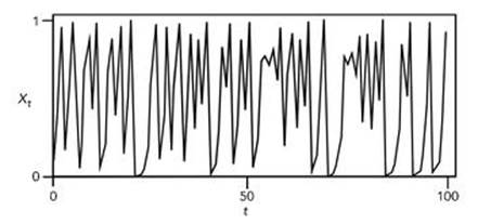
Fig 72 Chaotic behaviour in the discrete logistic model when a=4.
Although this model is too simple to be realistic, there is no reason why more complex models should not behave in similar ways, and there is plenty of evidence that they often do. So erratic changes in natural populations, previously attributed to irregularities in the environment such as changes in climatic conditions, can in fact be generated by the free-running dynamics of the population itself. May ended his paper with a call for such examples to be widely taught in schools, to prevent people assuming that irregular effects necessarily have irregular causes.
All well and good, but do real populations exhibit chaos? In the wild, it is difficult to separate a population’s own dynamics from the variations in environment that always occur in nature, so the occurrence of chaos has been controversial. Most of the data that zoologists and entomologists have collected over the years on animal and insect populations are seldom extensive enough to distinguish chaos reliably from randomness. The physical sciences get round such problems by performing controlled experiments in the laboratory, but even in the lab it is difficult to control the large number of extraneous variables that might affect experimental results in ecology. However, it’s not impossible.
In 1995 James Cushing and colleagues at the University of Arizona began a series of experiments that demonstrate the occurrence of chaos in populations of Tribolium castaneum, known as the flour beetle or bran bug because it often infests stocks of milled grain. Their theoretical model has three variables: the number of feeding larvae, the number of non-feeding larvae (plus pupae, and newly emerged adults) and the number of mature adults.5 The flour beetle and its larvae indulge in egg cannibalism: they eat the eggs of beetles in the same species, including their own. This behaviour is incorporated into the equations of the model.
Some of the experiments were performed under specially controlled conditions: beetles were removed or added to the population to mimic the mortality rates observed in the wild. Other experiments were not manipulated in this manner. To avoid genetic changes, the adult population was replenished from time to time from other cultures, maintained under strict laboratory conditions.
These experiments showed the expected onset of oscillations, but not chaos. However, the theoretical model can be chaotic, and the experimental system was quite close to the range of variables in which chaos occurs in the model. By changing the protocol to mimic a higher mortality rate than there would normally be in the wild, the same team managed to drive the beetle population into chaotic fluctuations.6 This second paper concludes:
The experimental confirmation of nonlinear phenomena in the dynamics of the laboratory beetle lends credence to the hypothesis that fluctuations in natural populations might often be complex, low-dimensional dynamics produced by nonlinear feedbacks. In our study, complex dynamics were obtained by ‘harvesting’ beetles to manipulate rates of adult mortality and recruitment. For applied ecology, the experiment suggests adopting a cautious approach to the management or control of natural populations, based on sound scientific understanding. In a poorly understood dynamical population system, human intervention ... could lead to unexpected and undesired results.
Chaos also solves the paradox of the plankton. The paradox is a violation of Gause’s principle of competitive exclusion: there are many more species of plankton than there are environmental niches. The plankton can’t be wrong, so there must be more to the principle than is usually thought. The question is, what?
There are well-established ecological models that agree with Gause’s principle. Ultimately, they trace the relation between the number of species and the number of niches to a general mathematical fact: if you have more equations to solve than you have variables, solutions don’t exist. Roughly speaking, each equation pins down a relation between the variables. Once you have as many relations as variables, you can find the solutions. Any extra equation is likely to contradict the solutions already found. As a simple case, the equations x+y=3, x+2y=5 are satisfied only when x=1, y=2. If we add a further equation, such as 2x+y=3, it is not valid for that solution. Only when the extra equation provides no new information will the original solution survive.
The competitive exclusion principle often works well, and since the mathematics supports it, ecologists have a puzzle on their hands.
Part of the answer is that the upper reaches of the Earth’s oceans are vast, and plankton are not uniformly mixed. But it now looks as though there could be a better explanation of the paradox of the plankton. The standard mathematical model makes a restrictive assumption: it seeks steady-state solutions to the relevant equations. The populations of organisms in the species concerned are assumed to remain constant over time; they can’t fluctuate.
This assumption in effect takes the ‘balance of nature’ metaphor for an ecosystem too seriously. Real ecosystems, if they are to survive for long, have to be stable. If the populations of various organisms fluctuate wildly, some may die out, and that changes the dynamics of the ecosystem. However, stability need not require the entire system to remain in exactly the same state for ever, just as a stable economy is not one in which everyone always has exactly the same amount of money as they did yesterday. The crucial feature of stability is that fluctuations in populations must remain within fairly tight limits.
Chaotic dynamics does precisely that. It exhibits erratic fluctuations, but the size and type of those fluctuations is determined by an attractor: a specific collection of states to which the system is confined. It can move around inside the attractor, but it can’t escape. In 1999, the Dutch biologists Jef Huisman and Franz Weissing showed that a dynamic version of the standard model of resource competition can produce regular oscillations and chaos if species are competing for three or more resources.7 In other words, as soon as the system is allowed to be out of equilibrium, the same resources can permit a much greater amount of diversity among the organisms that are using them. Roughly speaking, the dynamic fluctuations allow different species to utilise the same resources at different times. So they avoid direct competition not by one of them winning and killing off all the others, but by taking turns to access the same resource.
The same researchers, and others, have since developed these ideas into a wide range of models, and the resulting predictions are often in agreement with data from real plankton communities. In 2008, Huisman’s team reported an experimental study of a food web isolated from a natural one in the Baltic Sea, involving bacteria, plant plankton, and both herbivorous and predatory animal plankton.8 Their observations were carried out over a period of six years in a laboratory. The external conditions were kept exactly the same throughout, but the populations of the species concerned fluctuated significantly, often by a factor of 100 or more. Standard techniques for detecting dynamical chaos revealed its characteristic signs. There was even a butterfly effect: the future of the system remained predictable only a few weeks or a month ahead.
Their report remarks that ‘Stability is not required for the persistence of complex food webs, and that the long-term prediction of species abundances can be fundamentally impossible.’ And it refers back to May’s original suggestion that chaos could well be important for our understanding of ecosystems – a prescient insight that is now thoroughly vindicated.
Disease epidemics take place in a special type of ecosystem, involving both the organisms that become infected and the microorganisms – viruses, bacteria, parasites – that cause the disease. So similar modelling techniques, suitably modified, can be used for both ecosystems and epidemics.
In 2001 an abattoir in Essex reported that a consignment of pigs was suffering from foot-and-mouth disease. The disease spread rapidly, and the European Union slapped an immediate ban on the export of all British livestock. In all, there were two thousand outbreaks of the disease on British farms, leading to the culling of ten million sheep and cattle. The total cost was around £8 billion, and the news media showed piles of dead cattle being burnt in fields, a scene straight out of Dante’s Inferno that did little for public confidence. Was the strategy of stopping all animal movement within the UK, and slaughtering all animals on any infected farm, the right one?
Foot-and-mouth disease is caused by (several forms of) a virus that hardly ever affects humans, a picornavirus (see Figure 27, p. 141). But food is a very sensitive issue, so it would not be acceptable to let the disease spread. It also causes damage to meat and milk production, causes serious distress to the animals, and leads to import bans. So the standard response throughout the world is to eradicate it. Vaccination might become a viable and cheaper alternative. But even if the response is to slaughter infected animals, or those that soon might be, many different strategies for controlling the disease can be contemplated.
It is therefore important to decide which strategy is best. Mathematical modelling of the 2001 outbreak, after the event, suggests that initially the UK Government’s response was too slow; then, when the disease became widespread, it was too extreme. Only one animal in five among those slaughtered was infected. This overkill may have resulted from inadequate and outdated mathematical models for the spread of the epidemic.
Models are the only way to predict the likely spread of an epidemic and to compare possible control strategies. They can’t forecast which farms will be hit, but they can provide an overview of general trends, such as the rate at which the disease is likely to spread. In the 2001 outbreak, three different models were used.9 When the outbreak began, the main model available to DEFRA, the government department then responsible for agriculture, was a probabilistic one called InterSpread. This provides a very detailed model, farm by farm if need be, and includes many different routes for disease transmission. It might seem that the more realistic a model is, the better it will perform, but ironically InterSpread’s complexity is also its weakness. The calculations take a long time, even with powerful computers. And fitting the model to real data requires setting the values of a large number of parameters, so the model may be unduly sensitive to small errors in estimating these parameters.
A second model, the Cambridge – Edinburgh model, can also represent the location of every farm, but it uses a much simpler mechanism to model the transmission of the disease. Farms with the disease are ‘infectious’, those that are not yet infected but may come into contact with infected farms are ‘susceptible’, and the model combines all these variables to come up with an overall measure of how rapidly any given farm is likely to infect others. This model forecasts the geographical spread of the disease quite well, but its performance is poorer when it comes to the timing – perhaps because it assumes that the disease takes the same time to show up in all infected animals, and every animal remains infectious for the same period of time. In reality, these times vary from one animal to another.
The third model, the Imperial model, is based on traditional equations for the spread of epidemics, and was put together during the epidemic. It was less realistic than the other two, but much faster to compute, so it was more suitable for tracking the progress of the disease in real time. It predicted the changes in the number of infected animals, but not the locations of outbreaks.
Each model turned out to be useful for some types of forecast, and subsequent analysis suggests that, on the whole, the strategy of widespread slaughter was probably correct. It would not have been feasible to determine precisely which animals were infected during the rapid spread of the disease, and any infected animals mistakenly left alive would create new centres from which the disease could again spread, rendering previous actions useless. But the analysis also made it clear that the initial response was too slow. If more stringent restrictions on the movement of animals had been put in place immediately, and early cases spotted sooner, then the disease would not have had such a huge economic impact.
The second and third models also indicate that vaccination is not likely to be an effective control strategy once the disease becomes widespread, but vaccinating all animals in a ring surrounding an infected farm might restrict the spread of the disease if it is done right at the start.
These three models of the foot-and-mouth epidemic show how mathematics can help to answer biological questions. Each model was much simpler than any truly ‘realistic’ scenario. The models did not always agree with one another, and each did better than the others in appropriate circumstances, so a simple-minded verdict on their performance would be that all of them were wrong.
However, the more realistic the model was, the longer it took to extract anything useful from real-world data. Since time was of the essence, crude models that gave useful information quickly were of greater practical utility than more refined models. Even in the physical sciences, models mimic reality; they never represent it exactly. Neither relativity nor quantum mechanics captures the universe precisely, even though these are the two most successful physical theories ever. It is pointless to expect a model of a biological system to do better. What matters is whether the model provides useful insight and information, and if so, in which circumstances. Several different models, each with its own strengths and weaknesses, each performing better in its own particular context, each providing a significant part of an overall picture, can be superior to a more exact representation of reality that is so complicated to analyse that the results aren’t available when they’re needed.
The complexity of biological systems, often presented as an insuperable obstacle to any mathematical analysis, actually represents a major opportunity. Mathematics, properly used, can make complex problems simpler. But it does so by focusing on essentials, not by faithfully reproducing every facet of the real world.