Methods of Mathematics Applied to Calculus, Probability, and Statistics (1985)

Part II. THE CALCULUS OF ALGEBRAIC FUNCTIONS

Chapter 10. Functions of Several Variables

10.1 FUNCTIONS OF TWO VARIABLES

Up to now we have concentrated on functions of a single independent variable, and have used the notation

y = f(x)

We are often interested in phenomena that involve more than a single independent variable, and therefore we must examine functions of several variables. It is prudent to examine the case of two independent variables before examining the general case of n independent variables (Section 10.6).

The standard notation for functions of two independent variables is

z = f(x, y)

where x and y are the independent variables and z is the dependent variable. We think of the corresponding geometrical picture in three dimensions, the x and y mutually perpendicular axes horizontally, and the z variable is the third (perpendicular) direction upward. There are, unfortunately, two distinct such coordinate systems. Mathematicians generally use a left-handed one, shown in Figure 10.1-1a, and scientists and engineers often use a right-handed system, shown in Figure 10.1-1b. The names “left handed” and “right handed” come from the motion along the z-axis of a screw as you turn from the x-axis to the y-axis. It is unlikely that either group will, in the near future, abandon their system for the other, so you need to know both systems.

Plotting points in the three-dimensional (mathematical) space is straightforward; they are taken in the order (x, y, z). Thus the point P₁ with coordinates (1, 2, 3) is shown in Figure 10.1-1 along with the point P₂ with coordinates, (2, −1, 4). There is no widely used system for numbering the eight octants (corresponding to the four quadrants), and it is customary to give the signs of the three variables x, y, and z to indicate the octant you are talking about. All three coordinates positive is the first octant.

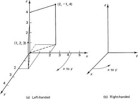
Figure 10.1-1

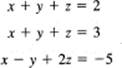
Once you can plot points, the next thing to consider is the distance between two points. Let the three coordinates be in the same units, and let the two points be P₁ (1, 2, 3), and P₂, (2, – 1, 4), of the previous paragraph. Think of them as the diagonal corners of a rectangular room whose sides are parallel to the coordinate axes (Figure 10.1-2). Using the Pythagorean distance, the square of the length of the diagonal on the floor is the sum of the squares of the lengths of the two sides,

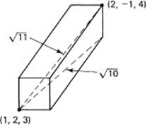
Figure 10.1-2 Distance between points

Now the vertical height of the room is measured perpendicular to the floor, and it is perpendicular to the diagonal line whose length we just computed. Applying the Pythagorean distance again, we find that the square of the room diagonal length is

d² = 10 + (4 – 3)² = 10 + 1 = 11

We immediately generalize; in the case of two general points, with coordinate subscripts 1 and 2, the Pythagorean distance between them is

Notice that (1) the distance function is symmetric in the three coordinates, (2) involves the squares of the differences of the coordinates, and (3) the points can be taken in either order (for any coordinate). In words, the square of the distance between the two points is the sum of the squares of all the differences of the corresponding coordinates of the two points.

We next turn to linear relations among the variables. The simplest general form is

Assume, for the moment, that C ≠ 0. We can therefore write the equation as solved for z,

z = ax + by + c

where the lowercase letters are related to the uppercase letters in an obvious way: a = −A/C, b = −B/C, and c = −D/C. For each pair x and y, this equation gives a corresponding z value, and the triple numbers (x, y, z) represents a point. The locus of all the points that satisfy the equation is a plane. The plane

z = x + 2y − 3

is drawn in Figure 10.1-3, and all you see are the traces on the three coordinate axes. The plane, of course, extends indefinitely in all directions, but the figure you see is the small triangle. The figure is easiest drawn by finding the intersections of the plane with the coordinate axes. To do this, you merely set each pair of variables equal to zero to find the value on the corresponding axis. Thus, in this example, to find the point on the x-axis, we set y = z = 0, and find that x = 3. Putting one letter equal to zero gives the equation of the straight line on the corresponding plane. For example, for x = 0 you have z = 2y − 3 in the y–z plane.

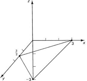
Figure 10.1-3 Plane z = x + 2y − 3

From your knowledge of lines in a two-dimensional plane, you see that linear equations in three variables represent planes in three dimensions without rigorously proving it. The special cases of a and/or b = 0 can be analyzed. For example, if both a and b are 0, then for all x and y we have z = c; it is a horizontal plane parallel to the x–y plane. If only one coefficient is zero, say a = 0, then the plane is parallel to the x-axis and cuts the y–z plane in the line (trace) defined by

z = by + c

when viewed as an equation in the y–z plane (see Figure 10.1-4).

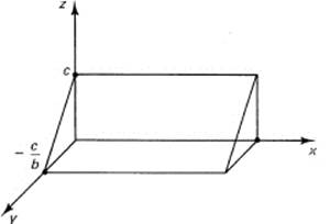
Figure 10.1-4 Plane z = by + c

A straight line is described by the intersection of two planes; it takes two constraints on the three variables to define a line. For example, the equations

z = 3 − x − y

z = 4 − 2x + 4y

together describe the locus of a line. The points of the line must lie on both planes at the same time.

But any point that satisfies both equations also satisfies any linear combination of the equations. For example, if you multiply the top equation by 4 and then add this to the lower equation, you eliminate the y variable. You have

5z = 16 − 6x

This is another plane through the same line defined by the two original equations. You could, instead, eliminate the x variable. Multiply the top equation by 2 and the lower by −1, and then add

z = 2 − 6y

These two derived planes equally well serve to define the line, and are somewhat preferable because you can see them more easily. The first plane is parallel to the y-axis and you see the projection of the line onto the z–x plane, while the second is parallel to the x-axis and you see the projection on the y–z plane (Figure 10.1-5). Thus the equations of a line are not unique; any pair of planes through the line will serve to describe it.

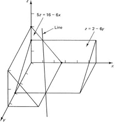
Figure 10.1-5 Two projections of a line

Generalizing the above, given the two equations that define a line, any linear combination of the equations also defines a plane through the line. This resembles the similar observation that, given two lines in two dimensions having a common point, then any linear combination of the two equations defines a line that also passes through the common point. And this probably brings to mind the warning that, just as two lines may be parallel and have no common point, so too may two planes be parallel and have no common line. Going further, you see that by picking a suitable choice of the constants you can form the linear combination that will define any line (plane) through the common point (line).

You could look at many special forms of the plane corresponding to the special forms of the line in two dimensions. The basic tool is the use of the general linear form (10.1-1) for a plane

together with the method of undetermined coefficients. Note that there exists an extra parameter (just as there did in the case of a line in a plane). For example, if D ≠ 0, then from this form by dividing by −D, and a little algebra, you can get the intercept form

of the plane. Inspection shows that the two equations

are the equations of a line through the points P₁ and P₂, and thus represent the two-point form.

Example 10.1-1

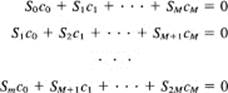
Given three points, say (1,1, 1), (2, −1, 3), and (1, 0, 2), determine the corresponding plane through them. We use undetermined coefficients and substitute the values of the points into the general form for the plane (10.1-3). From the three points, we get the following three conditions on the coefficients of the plane:

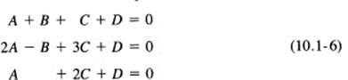
Their solution gives the coefficients of the plane through the three points. It is easiest in this particular system to eliminate B by adding the top two equations:

3A + 4C + 2D =0

Next, we take this with the third equation, and eliminate A by subtracting this from three times the third equation:

(6 − 4)C + D = 0

or

From the third of the original equations (10.1-6), we have

A = −2C − D = D − D = 0

Next, from the top equation of (10.6-6), we solve for B

Therefore, the equation of the plane through the three points is

Dividing out the D (as it must) and multiplying through by 2, we get, finally,

y + z = 2

This is a plane parallel to the x-axis. It is easy to check by direct substitution that this plane contains the three points.

Generalization 10.1-2

Linear Algebra. We have just solved three equations (10.1-6) in three unknowns, A, B and C. We have progressed to the point where from a single special case we can go to the general case. In this spirit we examine the general problem of solving three linear equations in three unknowns, x, y and z (we have changed from the unknown letters A, B, and C of the plane to the more usual variables x, y, and z). Let the given equations be

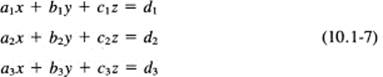
where we have adopted the usual notation of the independent variables as x, y, z, and the coefficients a_i, b_i, c_i, d_i are constants.

The method of solution we will use is known as Gauss (1777–1855) elimination. It systematically eliminates one variable at a time. We begin by supposing that at least one term in x is present, and it is no loss in generality to suppose this x is in the first equation, since we could renumber the equations if necessary. Thus we assume that a₁ ≠ 0. Multiply the top equation by −a₂, and add the equation to a₁ times the second equation. We have

This equation, together with the first original equation, is equivalent to the second equation, because the second equation can be reconstructed from the first equation plus the derived equation by a suitable combination.

Similarly, multiplying the top equation by −a₃, and the third by a₁, and then adding, you get

The original system (10.1-7) is now equivalent to the first original equation plus the two derived equations, (10.1-8) and (10.1-9) (since the steps are reversible). But the two derived equations depend on only two variables y and z. Repeating the elimination process, we eliminate the yterms and get a single equation in z.

Thus the original system is now equivalent to a triangular system of equations, whose solution is called the back solution of the Gauss elimination process. We are apparently led to a unique solution by this method of systematically eliminating one variable at a time.

What can go wrong? First, at each stage the method supposes that there is at least one equation in which the next variable to be eliminated appears. It might be that this is not the case. For example,

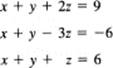
After eliminating x we will find that there is no y term in the two derived equations. The quantity x + y always occurs together and it is really not two variables. Thus, we cannot hope to determine x and y separately. This situation can arise when any two (or more) variables are coupled together. This situation means that one (or more) of the variables can be picked as we please; we can have infinitely many solutions of the system provided the rest of the solution process does not get into a contradiction, such as z = 6 from one equation and z = 7 from another equation.

A second thing that can go wrong is that at some stage all the variables in thé equation cancel out. For example,

Evidently, when we eliminate the x at the first stage between the first two equations, we will get

0 = − 1

which is a contradiction, meaning geometrically that the first two equations represent parallel, distinct planes that have no common line of intersection. If the second equation had been, for example,

2x + 2y + 2z = 4

then the elimination would have left us with

0 = 0

which means parallel coinciding planes, and hence the second equation represents no constraint on the variables other than that of the first equation. There are really only two equations defining the three variables, and one of the variables (say z if you wish) may be picked to be anything you please—leading to a one parameter family of solutions (a straight line).

This method of Gauss elimination can clearly be applied to n linear equations in n independent variables. The algebraic interpretations of what happens when you cannot go on are about the same; either a variable disappears completely from all the derived equations at that stage, or else all the variables in one equation drop out. The first shows a basic connection between the variables. The second implies a linear relationship between the involved equations; the equation that produced the row of zeros is a linear combination of the ones above. If the right-hand side is not zero, this means the equations are inconsistent (parallel distinct planes). If the right-hand side is equal to zero (coinciding planes), this means that at least one of the equations is redundant, and you have at least a one-parameter family of solutions.

EXERCISES 10.1

1.Find the plane through the three points (1, −1, 0), (0, 1, 2), and (2, 1, 1).

2.Find the plane through the three points (1, 1, −1), (1, −1, 1) and (−1, 1, 1)

3.Using the intercept form (10.1-4), find the plane with the intercepts 1, 2, 3.

4.Rewrite the general form of a plane (10.1-3) in a one-point form. Ans.: A(x − x₁) + B(y − y₁) + C(z − z₁) = 0.

5.What is the condition that a plane pass through the origin?

6.What is the condition that a plane be parallel to the z-axis?

7.Discuss the geometric situation where each of three planes can intersect the other two but that there is no common point of the three planes.

8.Give the condition that two planes be parallel.

9.Draw the plane x + y + 3z = 5.

10.Draw the plane 2x − y − 2 = −2

11.Draw the planes x + y + z = 1 and x − y + z = −1 and sketch the line.

12.Find the equations of a line through (1, −1, 1) and (1, −2, 3). Hint: Use Equation (10.1-5).

13.Solve the system of equations x + y = 3, y + z = 4, z + x = 5. Generalize.

10.2 QUADRATIC EQUATIONS

In Euclidean geometry (see Figure 10.2-1), the Pythagorean distance in three dimensions (all of the same kind, and not “apples plus oranges”), is given by the formula (10.1-2):

d² = (x₂ − x₁)² + (y₂ − y₁)² + (z₂ − z₁)²

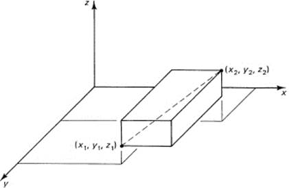
Figure 10.2-1 Distance

It is easy to recognize that if r is a fixed number then the equation

is the equation of a sphere about the point (x₁, y₁, z₁) of radius r (we have set d = r for convenience of calling the distance the radius of the sphere). Thus, there is a close analogy between circles in the plane and spheres in three dimensions; for example,

x² + y² = 1

is a circle of radius 1 about the origin in two dimensions (arid in three dimensions this would be a cylinder of radius 1 about the z-axis). Again,

x² + y² + z² = 1

is a sphere of radius 1 about the origin in three dimensions. Clearly, the trivial plane cuts the sphere in the circle

Planes clearly cut a sphere in circles, although the intersection of a tilted plane with a sphere requires some attention to prove that it is a circle.

When we go to three variables, and examine the general equation of degree two in three variables, we will have three-dimensional conics.

By suitable rotations in each plane, the cross products xy, xz, and yz can be removed (Section 6.9*) and the general form reduced to

Of course, the A, B, … have been changed from their original values when we make the rotation, but it is convenient to use the same letters.

The complete analysis of the general case (which involves the completing of the squares of the quadratic variables to gain symmetry) will be omitted, and we will examine only a few special cases. An ellipsoid is of the form

Notice how this extends the idea of an ellipse, just as the distance in three dimensions extended the two-dimensional distance and the sphere extends the idea of a circle (see Figure 10.2-2). In particular, when a = b = c, the ellipsoid will be a sphere whose radius is the common value of the three coefficients. When only two of the coefficients are equal, it is an ellipsoid of revolution about the nonequal axis (Figure 10.2-3); oblate when the equal axes are the larger, and prolate when they are the smaller of the axes.

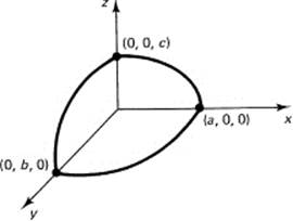
Figure 10.2-2 Ellipsoid

For the corresponding hyperboloid, there are two cases. The hyperboloid of one sheet (one connected piece) occurs when there is one minus sign among the squares of the three coefficients on the left-hand side; for example,

(see Figure 10.2-4). The hyperboloid of two sheets (two separate pieces) has correspondingly two minus signs,

Figure 10.2-3 Prolate spheroid

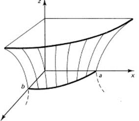
Figure 10.2-4 Hyperboloid of one sheet

(see Figure 10.2-5). Three minus signs would, of course, produce an imaginary locus, since the left-hand side would then be negative (for real numbers x, y, and z, as well as real numbers a, b, and c), and the right-hand side is plus 1. Only complex (imaginary) coordinates could satisfy the equation.

In a similar way, there are paraboloids, hyperbolic paraboloids, elliptic paraboloids, and even cases when only one term is quadratic. They will occur now and then in the text as examples, but each time the meaning can be deduced as needed rather than examined now, and promptly forgotten!

Further development of the theory is now well within your abilities (chiefly completing the square on the quadratic variables and translating the coordinate system), but the number of special cases is naturally much larger (there are said to be 17 distinct cases!).

Instead, let us discuss how to draw the surfaces. Most of the time the coordinates have been chosen so that what symmetry there is occurs with respect to either the coordinate planes or coordinate axes. This is often referred to having the surface as a central conic. We then find the traces of the surface on the coordinate planes. To do this for the x–y plane, we simply set z = 0. The problem is thereby reduced to the two-dimensional problem of earlier chapters. Similarly, we set y = 0, and find the trace on the x–z plane. Finally, we set x = 0 and find the trace on the y–z plane. If the figure is not obvious from this, then we can try sections (cross sections) through the surface. For example, putting z = 5 gives the cross section of the surface parallel to the x–y plane at the height z = 5. Similar cross sections in other planes generally will fill in the surface enough for you to draw a reasonable sketch of it.

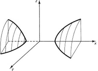
Figure 10.2-5 Hyperboloid of two sheets

Example 10.2-1

Draw the surface

x² + y² − z² = 1

You immediately see that there is symmetry with respect to all three coordinate planes (replacing any variable by its negative does not change the equation; hence, if any coordinate satisfies the equation, then its negative also satisfies the equation). For z = 0, the trace in the x–y plane gives you a circle of radius 1. You can also see that as z gets larger the circle in the intersection plane parallel to the x–y plane grows in radius (r² = 1 + z²).

Next set y = 0. In the x–z plane you have a hyperbola with 45° asymptotes. And similarly, in the y–z plane. You are ready to draw Figure 10.2-6, which is a hyperbola of one sheet.

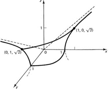
Figure 10.2-6 x² + y² − z² = 1

Example 10.2-2

Draw the surface

x² − y² + z = 0

From the squared terms you see the symmetry in the y–z and x–z planes. The trace on the x–y plane (z = 0) is a pair of straight lines, y = ±x. The trace on the x–z plane is a parabola opening downward, while the trace on the y–z plane is a parabola opening upward. This saddle shape is hard to sketch clearly (see Figure 10.2-7). It has the general shape of a pass between two mountains.

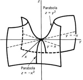
Figure 10.2-7 Hyperbolic paraboloid saddle

Example 10.2-3

Draw the surface

z = x²

In this equation the y does not occur, so you get the same pair of (x, z) for each y. From the x² term you see the symmetry with respect to the y–z plane. It is a cylindrical surface along the direction of the y-axis. The trace is a parabola in the x–z plane. See Figure 10.2-8, which is a parabolic cylinder.

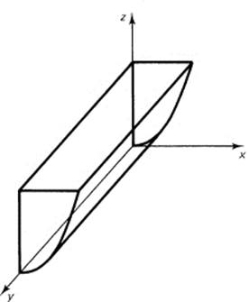
Figure 10.2-8 cylinder z = x²

EXERCISES 10.2

1.Write the equation of the sphere centered at the origin with radius 4.

2.Write the equation of the sphere with center at (0, −3, 4) and radius 5.

3.Find the center and radius of x² + y² + z² − 2x − 4y + 6z = 11.

4.Find the center and radius of x² + y² + z² − x + y + 3z = 0

5.Sketch the first octant of the surface x² /4 + y² + 4z² = 1.

6.Sketch x² − y² + z² = 1.

7.Sketch x² + y² −z = 0.

8.Find the sphere through the four points (0, 0, 0), (0, 0, 1), (1, 0, 0), and (0, 1, 1).

9.Plot x²/4 + y²/9 + z²/25 = 1.

10.Plot y² = x.

10.3 PARTIAL DERIVATIVES

We have repeatedly used plane sections of the surface to find the nature of the surface. This amounts to assigning a fixed value for one of the variables. Suppose we fix the y variable, set y = c. But y = c is the equation of a plane and it cuts the surface in a plane section. If we use the calculus to study the curve in this plane, then we will want to take derivatives. But this could be confused with the derivatives in just two variables. Thus we have to use a different notation for the letter d; we use one form of the Greek lowercase delta

when we write the symbol of the partial derivative of z with respect to x. Similarly, fixing the value of x, we have the partial derivative of z with respect to y.

The confusion arises in some student’s minds when the choice of the fixed value, the y = c, is allowed to vary. Consider the function

z = xy²

We have

In each case you regard only the indicated variables as changing. These derivatives depend on the point where they are evaluated, the x and y coordinates, and they are the slopes in the corresponding planes parallel to the coordinate axes. Higher derivatives are similarly defined.

There are cross derivatives, and it is an important fact that for most functions you are apt to meet (but not for all functions) the order in which they are taken is not important.

In the above equation, z = xy², the cross partial derivative is 2y. We will not prove this fact here, but several examples will convince you of its truth in simple cases. Pathological functions can be found for which it is not true, but for the class of functions we generally meet the cross derivatives are equal.

Example 10.3-1

For the general conic (10.2-2), there are cross-product terms in the equation; hence the cross derivatives are not identically zero. Cross derivatives can be other than 0 only when the corresponding term depends on both variables. For a term like

z = x^myⁿ

we have

whether we do the x or y differentiation first.

The implicit differentiation of Section 8.3 can now be seen in another light. Suppose you have an equation in two variables,

f(x, y) = 0

Differentiating this with respect to x, you have from basics

But this can be written as [subtract and add the term f(x, y + y)]

We divide this by Δx, and then take the limit as both x and y go to zero. In the first two terms, the second argument is the same, so we have a partial derivative with respect to the first variable. In the second pair, it is the first argument that is the same, so we multiply and divide by y and then take the limit. Thus we get

From this you have

This is the same thing as you had earlier from implicit differentiation, but with a new notation.

Example 10.3-2

Using the third example in Section 8.3, we have

z = f(x, y) = x²y² + 5y − x⁴ − 5

Find dy/dx. The partial derivatives are

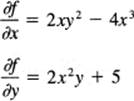
from which, using Equation (10.3-2), you have, again,

EXERCISES 10.3

Find the first partial derivatives and the cross derivative of the following:

1.z = x² + y²

2.z =

3.z = x/y

4.z = x²y + y²x

5.z = (x − y)/(x + y)

6.Find the tangent plane to the sphere x² + y² + z² = 1 at the point Hint: Use Ax + By + Cz + D = 0;equate the value and the two partial derivatives of the two surfaces at the given point.

10.4 THE PRINCIPLE OF LEAST SQUARES

Up to now we have been dealing with mathematical objects having mathematical definitions; our points, lines, planes, curves, and surfaces were exact. But everyone knows that when you measure things in the real world you find that the measurements are not exact, that there is noise added to the true value, whatever “noise” and “true value” may mean! You think there is a true value, say x, but when you make the nth measurement, you get ( is the lowercase Greek epsilon)

where _n is the corresponding error in the measurement. The quantity _n is called the residual at n. For N measurements, you have the index n running from 1 to N.

Given a number of measurements x_n, what value should you take as the best estimate of x? The principle of least squares asserts that the best estimate is the one that minimizes the sum of the squares of the differences between your estimate and the measured values. That is, you minimize the sum of all the terms

as a function of x. This is exactly the same as the sum of the squares of the residuals:

We write this more compactly as (see Section 9.9)

This compact notation carries a lot of details, and you should frequently ask yourself what the expanded version of the summation really looks like so that you will realize how much is being done with this summation notation. Being compact, it allows you to think in larger units of thought (chunks), to carry things further along, without the excessive effort of watching all the details.

This function f(x) is a function of the single variable x. To find the minimum, you naturally differentiate with respect to x and set the derivative equal to zero. You get (each term in the summation differentiates the same)

The original function was a parabola in x, so you believe that this equation gives the minimum (and you also have d²f/dx² = 2N > 0). You have, since the sum of the terms in the parentheses of this sum can be added separately (due to the linearity of the operator ),

The second summation is a common occurrence; the quantity x being summed over the N terms does not depend on the index n. There are N copies of x to be added, and you get for the second sum

Nx

To solve for x, divide the equation by N:

which is simply the average of all the observations. This is also called the mean value of the observations. The average of all the observations is the least square estimate (according to the least squares principle).

Example 10.4-1

Given the seven observations

3.1, 3.3, 3.1, 3.2, 3.3, 3.1, 3.5

we add them to get the sum 22.6. If we now divide by the number of observations (N = 7), we get

as the least squares fit to the data.

There are a number of simple shortcuts when doing this mentally (and they are sometimes useful on a computer to save accuracy). First, note that for these data the first digit is always 3, and we can ignore it provided we later compensate by putting it back. Next, instead of regarding the rest of each number as a decimal, we can imagine it multiplied by 10, so we can deal with the seven integers, 1, 3, 1, 2, 3, 1, 5. The sum is 16, and the average is . This is to be divided by 10 to compensate for making the numbers into integers, and then the initial digit 3 that we set aside is to be added. We get the same result as before:

Abstraction 10.4-2

The above simplification of the arithmetic is a general principle. Given N observations x_n, they can each be written as

where a and b are convenient numbers; typically, b is a power of 10 and a is near the mean of the observations.

When we take the average (mean) of the N observations x_n, we get

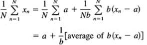
This is an extremely useful result not only for mental arithmetic, such as computing grade averages in your head, but also in large computing machines to keep accuracy.

EXERCISES 10.4

Find the least squares estimate of the following data:

1.5.1, 5.3, 5.2, 5.0, 4.9

2.−3.7, −3.9, −3.5, −3.6, −3.6

3.−5.1, −4.7, −5.2, −4.8, −5.3, −5.3, −4.9

10.5 LEAST SQUARES STRAIGHT LINES

Often you have N observations y_n, each observation depending on a corresponding x_n. In mathematical notation you are given the N data points

The x_n values are assumed to be correct, and the errors are in the y_n values. From a look at a plot of some data (Figure 10.5-1), the data seem to lie on a straight line. Suppose you try to fit a straight line to the data as best you can. Using the principle of least squares, you pick that line for which the sum of the squares of the differences (residuals) between the data at x_n and the value on the line at x_n is minima. Thus the sum of the squares of the residuals, the squares of the differences between the y values on the line, and the given values at x_n is to be made minimal.

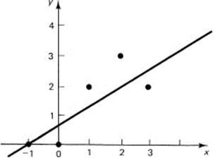
Figure 10.5-1 Least squares line

To get things in more mathematical terms, you want to fit the straight line

y = mx + b

to the N data points (x_n, y_n). The value on the line at x_n is the corresponding y (x_n) value from the line; that is, y (x_n) = mx_n + b. Thus the difference between the observed data y_n and the value from the line y (x_n) = mx_n + b is

where the error _n is the residual at x_n. The error is considered to be noise in the original measurements y_n. According to the principle of least squares, the sum of the squares of the residuals is to be minimized; that is,

This is a function of two variables m and b. This often comes as a surprise to the student: the constants of the line have become the variables! But consider the problem, “Which line is best?” The particular line you choose depends on the choice of the parameters m and b. They are the variables, and the x and y have been summed over all their values. It is necessary to belabor this point; the variables of the problem are the coefficients of the line. You are searching for the best line.

As a function of m and b, you can write it as

and you see that f(m, b) is a paraboloid in the independent variables m and b. If you set the partial derivatives of f(m, b) with respect to each of these variables (m and b) equal to 0, you will be led to the minimum. You have to differentiate each term in the sum, one by one. You get

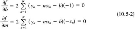
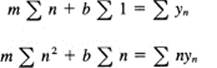
Since the right-hand sides are all 0, you can ignore the −2 factors that always arise. Next break up the sum of the terms of (10.5-2) into sums over each term:

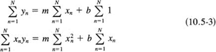
These equations are called the normal equations because they normally occur, and with familiarity you learn to write them down directly, if you do the least square fitting of polynomials often enough! If you don’t, then you remember the derivation of the normal equations: set up the sum of the squares of the residuals; then differentiate with respect to each of the parameters of the curve you are fitting and set equal to zero, and finally rearrange the equations.

When you compute the sums, which refer to the measured data, you will have two linear equations in the unknowns m and b to be solved. When solved, you will know the values of m and b for the least squares straight line that fits the data.

Example 10.5-1

Suppose you have the data given in the x and y columns of Table 10.5-1. The choice of very simple integers allows you to follow easily what is going on. In practice, of course, the numbers can be very awkward and require at least a hand calculator to carry out the arithmetic easily. To get the sums, it is best to make a table like Table 10.5-1.

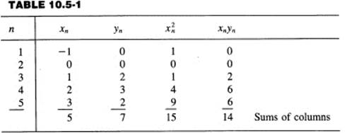
The normal equations (10.5-3) become, when these numbers are substituted for the sums,

7 = 5m + 5b

14 = 15m + 5b

(the 5 in the 5m term in the top line arises because the sum of the x_n is 5, and the 5 in the 5b because there are exactly 5 data points; while the 5 in the bottom equation is again the sum of the x_n). To eliminate b, subtract the top equation from the bottom:

7 = 10m

or

Next, you get from the top equation after substitution for m and some algebra,

The equation of the least squares line fitting the given points is

In Figure 10.5-1 you can inspect the results where both the data and the line appear. It is only by chance that the line goes through a given point. It does look like the proper choice since any changing of position vertically, or the slope, or any combination of the two, does not appear to reduce the sum of the squares of the errors (the vertical distance between the point and the line, not the perpendicular distance as you might suppose). Remember what the residuals are and what you minimized!

Generalization 10.5-2

Let us generalize the method. You are given N data points (x_n, y_n) and you have a model, in this case the straight line (y − mx + b). You want the least squares fit of the model to the data. You form the sum of the squares of the residuals and set out to minimize this as a function of the parameters of the model (the coefficients of the straight line). When the coefficients appear in the model in a linear fashion, as the m and b do for the straight line, then following through the partial differentiation to find the minimum, you see that the parameters will always occur linearly in the normal equations. You solve these linear equations, and if you care about the result, you plot the original data and the computed model (the straight line). Finally, you think carefully whether or not you would be willing to act on the results.

Example 10.5-3

We could go on fitting specific data by the model of a straight line to give you more exercise; instead, we will only partially abstract the problem in another direction and suppose (a very common situation) that the data at a set of N equally spaced values of x_n are simply y₁, y₂, …, y_N. The table for the sums is:

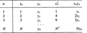
where we have assumed that the x values were at the integers. From Table 2.5-1 we know the sum of the first N integers and the sum of the squares. They are

We have, putting the summations involving y on the right-hand side,

where we have abbreviated the notation but what is meant is clear. The sums on the left-hand side are given immediately above, so we have only to solve for m and b to have the least squares straight line fitting the given data. In any specific case, we generally take the trouble to plot the points and the computed straight line to see if we have made any arithmetic mistakes along the way. You should also see if you like the result of assuming the criterion of least squares; when the result obtained is not reasonable and pleasing, then maybe it was the criterion of least squares that was inappropriate! It is generally a good idea to plot the residuals to see if there is any strange pattern in them.

Fitting a least squares line may be regarded as trying to remove the “noise of the measurement” from the data, “smoothing the data” if you prefer those words. It rests directly on the assumption that the best fit is that which minimizes the sum of the squares of the errors in the measurements y_n (and which also assumes that the x measurements are exactly right). Since least squares is so widely used, we had better examine this assumption in more detail. There is a saying that scientists and engineers believe that it is a mathematical principle and that mathematicians believe that it is a physical principle. It is neither; it is just an assumption. And although it can be derived from other assumptions (as we will in Section 15.9), in the final analysis it is an assumption, and not a fact of the universe. What is a fact is that when the parameters of the model occur in a linear fashion then the resulting equations to be solved are linear in the unknown coefficients, and hence are easily solved. This is what accounts for much of the popularity of the method.

What is wrong with the least squares is easily stated: it puts too much weight on large errors. A single bad data point can greatly distort the solution. Thus, given 100 observations, a single errror of size 10 (whose square is 100) has greater effect than 99 errors each of size 1. As a result of this, it is customary to inspect the data for outliers before applying least squares methods (and to inspect again, via the residuals, after the fitting).

EXERCISES 10.5

1.Examine the theory of fitting a straight line when there are an odd number 2N = 1 of points symmetrically spaced about the origin.

Find the least squares line through the following data:

2.(0, 2), (1, 1), (2, 2), (3, 0), (4, 1).

3.(−2, 2), (−1,1), (0, 0), (1,−1), (2,−2)

4.(−2, y₋₂), (−1, y₋₁, (0, y₀), (1, y₁), (2, y₂)

5.In Example 10.5-3, suppose the data were at x = 0, 1, …, N − 1. What changes would be necessary?

6.Carry out Example 10.5-3.

10.6 n-DIMENSIONAL SPACE

In Section 10.5, the fitting of a straight line to some data takes place in twodimensional space, the space of the coefficients of the straight line. Suppose we had tried to fit a parabola,

y(x) = ax² + bx + c

which has three coefficients, to some data; we would have to fit the data in the space of the three coefficients. The data (x_n, y_n) are in a two-dimensional space, but the fitting of the coefficients a, b, and c takes place in a three-dimensional space.

Now, suppose we tried to fit a polynomial having four coefficients. I say we would have to do the fitting in a four-dimensional space of the coefficients (parameters). And you see where we are headed.

As a specific example, suppose that the design of something, say an airplane engine, depended on 17 different parameters: the diameter of the rotor, the length of the blades, the number of rings of blades, and so on. The design would take place in 17-dimensional space. Of course, the engine is built in 3-dimensional space, but the design takes place in the space of the parameters, one dimension for each parameter. Do we mean a “real physical space”? No, what we mean is that you must give 17 different numbers to describe a single design. Each design is an ordered array of the 17 specific numbers. It is natural to regard this array of 17 numbers,

(x₁, x₂, x₃, …, x₁₇)

as a point in space. (We are now using x_m as the name of the mth variable.) We can imagine holding all but one of the variables fixed and varying that one, let it be the ninth. With the other 16 held fixed, we have the concept of the partial derivative and can imagine searching for the optimum value of x₉.

In going from three- to four-dimensional space, the student often struggles with the concept, trying to imagine, perhaps, if time is the fourth dimension. This is needless worrying and is the reason we have jumped so rapidly to 17-dimensional space. With 17 dimensions there is simply no question of asking if the space is “real” or not. Careful thinking will show you that we are being formal when we say that two variables led to two-dimensional space, that three variables is equivalent to three dimensions. The modeling of the mathematical formulation to common experience is so close that the student feels comfortable with the two- and three-dimensional mathematical models, but they are only models after all! Similarly, given 17 parameters (coefficients), we think of them as being modeled by a 17-dimensional space; each particular set of the 17 parameters is a point in the space, just as before each pair (or triple) of numbers was a point in two- or three-dimensional space. You have plotted three-dimensional figures on a two-dimensional plane, and not let that bother you very much.

Let us, for the moment, return to the example of N measurements of the same thing. We could adopt an alternative view and think of these N numbers from the measurements as a single point in N-dimensional space if we wished. This is quite a different space than the space of the coefficients of the line we fitted to the set of pairs of observations (x_n, y_n). The idea of an n-dimensional space is very fundamental to many mathematical ways of looking at things. It is a very useful concept, which requires gradual mastery since it can often provide a simple, familiar way of looking at a new situation that involves N numbers or M parameters. Both views lead to the concept of an n-dimensional space; one is that it is an N-dimensional space of the data, and the other that it is an M-dimensional space of the coefficients.

In the method of undetermined coefficients, we set up the criterion we want to meet, at present the least squares criterion, and find the coefficients by some means—in least squares by solving the normal equations. It is important to note that in least squares it is the linearity of the coefficients, not the terms they multiply, which assures you that the resulting normal equations will be linear in the unknowns.

The N measurements of the experiment often have very different kinds of dimensions (feet, weight, etc.), and we therefore are in a nongeometric space where rotations are meaningless. But it is convenient to keep the language of space when talking about the design. There is little meaning for slant distances between points in such a space, but there is meaning to distances between values of the same parameter. We can measure along the coordinate axes, but not diagonals (if we wish to keep much sense in what we are doing).

On the other hand, often the values in the space have a common unit of measurement, such as N measurements of the same thing. In such a space the Pythagorean distance between points can be very useful. We can say how far one set of N measurements that you may have made are from another set of N measurements of the same thing I may have made; after all, we do not expect them to coincide, and the distance between them gives some indication of the consistency between our measurements. It is dangerous, although unfortunately all too common, to use the Pythagorean distance when the units are not comparable. Least squares is related to the Pythagorean distance, but the distance function implies homogeneity of the units that are being added together to get the total distance. Sometimes a suitable scaling can make them the same. For example, in the special relativity theory the three distance units are made comparable to the time unit by using ict in place of t (c being the velocity of light and ) because the dimension of ct is (distance per unit time) × (time) = distance, and is therefore comparable with the distance units of the other three variables. The is not so easily explained!

The idea of n-dimensional space is simply a large generalization of our ideas of one-, two-, and three-dimensional spaces. When you think carefully about it, then the lower-dimensional spaces are seen to be no more “real” than the higher-dimensional spaces. It is just that you feel that the physical experiences from which you abstracted your ideas of the spaces are close by; they are easy for you to visualize. But the mathematical spaces of one, two, and three dimensions exist only in the mind, and as such are no more, nor less, “real” than the higher-dimensional mathematical spaces. There is an inevitability of higher-dimensional space, and you might as well get used to the idea.

Example 10.6-1

Suppose we tried to fit the special cubic (one parameter, M = 1)

y = ax³

to the following five data sets, (−2, −3), (−1, 0), (0, 0), (1, 2), (2, 4), using the principle of least squares. We first write the residuals

and sum their squares over all the data. We have

Differentiate with respect to the variable a and set the derivatives equal to zero to find the minimum:

From this we get

or

We now plot the result, y = 26x³/65, in Figure 10.6-1. It looks reasonable.

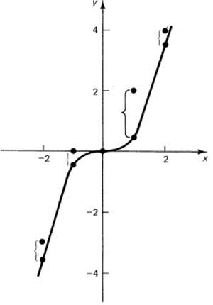
Figure 10.6-1 Least squares cubic

Example 10.6-2

To illustrate the use of a higher-dimensional space, we will fit a cubic (having four parameters, coefficients) to some symbolic data (x_n, y_n) for n = 1, …, N, using the criterion of least squares to choose the particular cubic from the family of all possible cubics. In mathematical symbols, we want to fit

y = c₀ + c₁x + c₂x² + c₃x³

to the data. “Least squares” means that we set up the sum of the squares of the residuals as a function of the parameters c₀, c₁, c₂, and c₃.

But _n is the difference between the observed data y_n and the corresponding value y (x_n) of the cubic (the model). Hence

where we have clearly shown that the variables are the coefficients of the equation. To find the minimum, we differentiate F(c₀, c₁, c₂, c₃) with respect to each parameter in turn, equate each to zero, divide out the −2, and finally transpose things to get the normal equations (c₀, then c₁, etc.). To avoid a lot of writing, we use the notation

The normal equations are, in this notation,

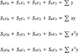
We need to make a table (corresponding to Table 10.5-1) of values, but with many more columns. We need the sums of the powers of the observed x_n up through the sixth power, and the sums of the data multiplied by the powers of x up through the third power. With even a small programmable hand calculator (let alone a large computer), this is not a great effort. Once they are substituted into the equations, we have four equations in four variables to solve. Again, from generalization 10.1-2, it is tedious, but not difficult, to do.

It is important that you understand what is going on; then when you face a practical problem you will know what to do even though it may take time. Normally, it takes many hours to gather some data, at times even years, and the effort to fit a least squares model to the data is trivial in comparison. Data gathering is expensive and data processing is relatively cheap. Indeed, routines for curve fitting of the above type are in standard statistical packages available on most computers. You know what the routine should be doing. If you take the trouble to plot the results (and the residuals) and examine it with a jaundiced eye, then you can catch most errors in either the way you used the statistical package or else in your application of the criterion of least squares. The final criterion is simply, “Are the results reasonable?” If not, why not? Is it the data, an error in arithmetic or algebra, or is it the peculiarity of the least squares method that puts great emphasis on large errors?

Example 10.6-3

To make sure we understand the general case, we will fit a cubic (M = 4) to nice integer data (N = 7). The equation is

y = c₀ + c₁x + c₂x² + c₃x³

The data are in the first two columns of Table 10.6-1.

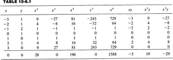
The normal equations are, therefore,

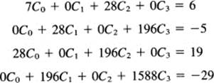
Due to the symmetry of the data points x_i these equations fall into two systems of two equations each. The first and third equations are one pair:

To solve them, multiply the top equation by −4 and add to the bottom equation to get

From the top of the pair, we have

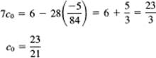
Similarly, we solve the second pair of equations, the second and fourth equations.

Multiplay the top of these two equations by −7 and then add to the lower equation to get

The solution is, therefore,

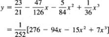
and is shown in Figure 10.6-2.

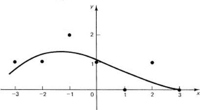
Figure 10.6-2 Cubic fit

Abstraction 10.6-4

Linear Algebra. The purpose of this abstraction is to show, using some conventional mathematical ways of thinking, that the normal equations that arise in polynomial fitting can always be solved in principle because they are linearly independent.

The method for proving that the normal equations have a solution is to show that the corresponding homogeneous set of equations (i.e., with the right-hand sides set equal to zero), have no solution other than all O’s. We study, therefore, the homogeneous equations in M + 1 variables c_i with S_m = ∑ x^mk

as the set of equations to be solved. Multiply the top equation by c₀, the second by c₁, …, the last by c_M, and add. You will get the squares of each c_i plus twice the cross products c_ic_j. When you follow out the details and write the S_i as sums, you will find that you have

The quantity in the braces is a polynomial of degree M, say P_M(x). This polynomial of degree M is evaluated at N > M + 1 points (more points than parameters or else it is not least squares). If the sum of the squares is to be zero, then each term of the sum must be zero since each term is nonnegative. Therefore, the expression in the braces must be zero for all N values of n. But a polynomial of degree M can only vanish at M distinct points. Said in other words, the powers of x are linearly independent; hence no linear relationship can exist among the terms other than with all zero coefficients. Therefore, the polynomial is identically zero; all its coefficients are zero. Thus the system of homogeneous equations has only the all zero solution.

We next apply the following general theorem, which we will prove shortly (note the change in notation):

Theorem. If n homogeneous equations

have only the solution of all zeros, then the nonhomogeneous equations

have a single solution.

From this theorem it follows that the complete system of normal equations as originally given has a unique solution, and the system of equations can be solved easily (in principle). There can be no trouble because the process cannot lead to multiple or inconsistent solutions. (Note that there can be roundoff trouble, however.)

It remains to prove this important theorem. When we passed from the n original nonhomogeneous equations to the n homogeneous equations, we moved each plane (corresponding to its equation) parallel to itself so that it finally passed through the origin. (The partial derivatives on each plane remained the same.) The theorem assumes that these homogeneous equations have only the single solution, which is the origin. We have now to get back to the solution of the original nonhomogeneous equations.

We first observe that the original n equations could have no solution, one solution, or infinitely many solutions. Suppose for the moment that the original nonhomogeneous equations had two different solutions; call them Y and Z. Each capital letter is the whole set of n numbers that constitutes the solution. Then the difference

U = Y − Z

(this is a symbolic equation indicating differences of solution values taken term by term, u_i = y_i − z_i, i = 1, …, n) will satisfy the homogeneous equations. To see this, we merely take any equation of the original set, say the first one,

put the Y values into this equation, then put the Z values into this same equation, and finally subtract. You see the U values on the left side and the cancellation of the b₁ on the right, leaving a homogeneous equation with the same coefficients. Since the homogeneous equations were assumed to have only the all zero solution, it follows that the nonhomogeneous equations cannot have two distinct solutions.

It remains to show that the nonhomogeneous equations have exactly one solution when the homogeneous equations have a single solution (which must be all zeros). Each equation defines a plane (sometimes called hyperplane). Consider one of these n equations, say the last one. The other n − 1 planes intersect in a line. This line pierces (intersects) the last plane in one point by the assumption that there is a single unique solution. Thus the n − 1 equations cannot have more than a line in common or else the intersection with the last plane would be more than a point, or else no points at all (in case the line is parallel to the chosen plane). Now we move the last plane parallel to itself back to its original position. The unique intersection will persist, although the values of the coordinates may change.

In a similar fashion, we move each plane back to its original position. In each case the movement may change the coordinates of the intersection, but cannot destroy the fact of a unique intersection.

For those who prefer algebraic to geometric arguments, we consider the same question in terms of the Gauss elimination (Generalization 10.1-2) applied to these equations. We will come down to a triangular system if all goes right, and if anything goes wrong and we do not get the triangular system, then the equations are either inconsistent (no solution) or else redundant (many solutions). But the Gauss reduction method operates only on the coefficients on the left-hand side of the equations and carries the corresponding right-hand sides along. The assumption that the homogeneous equations have a unique solution indicates that all the stages of the elimination went along properly and nothing went wrong. Supplying the appropriate right-hand sides in the triangular system, we get a unique back solution to the original system of equations. Thus we see that again the algebra and geometry agree, that each illuminates the other.

EXERCISES 10.6

1.Fit a quadratic y = ax² to the data of Example 10.6-1.

2.Write out the normal equations for fitting a fifth-degree equation as in Example 10.6-2.

3.Outline the proof that you can always solve the normal equations in the case of polynomial fitting.

10.7 TEST FOR MINIMA

We have been assuming that a minimum was found by equating the M + 1 partial derivatives to zero (corresponding to the M + 1 parameters c₀, c₁, …, c_M). Since we were forming a quadratic expression in the parameters (which is the surface in the M + 1 dimensions we are exploring for a minimum), we see that there is a unique minimum, and that at this minimum point the partial derivatives must be all zero (or else we could move in some direction to decrease the value of the sum of the squares of the residuals). We are effectively asserting that for this surface the minimum occurs where for each plane section with all other variables held fixed there is a minimum in this plane. Thus to find the minimum we compute the partial derivative in the plane and equate the partial derivatives to zero to define the unique minimum. This is true in this special case, but you should be wary of this approach in general, as the following classic example shows.

Example 10.7-1

Consider the simple z surface with two independent variables x and y:

z = (y − x²)(y − 2x²) = y² − 3x²y + 2x⁴

Let us look at a plane section made by a plane through the z-axis. Such planes have the form

y = cx

On this plane we have

z = c²x² − 3cx³ + 2x⁴

and we have

at the origin. The second derivative at x = 0 is

Thus, except when c = 0, this is a guaranteed minimum on this plane. For c = 0, we have the cross section in the plane

z = 2x⁴

and on this plane we know that the origin is a local minimum,. Finally, we take the plane that goes along the y-axis (x = 0). We have

z = y²

and again it is a local minimum. To summarize at this point, every plane section containing the z-axis gives a local minimum. Yet when we look at the picture from above (Figure 10.7-1), we see the x–y plane and the two curves along which z = 0; that is,

y = x² and y = 2x²

We also see that between the two parabolas the function must take on negative values! Note that the factor y − x² is positive and y − 2x² is negative in the curved region between the two parabolas. The origin is not a local minimum; there are negative values of the function in the immediate neighborhood, no matter how small, of the origin.

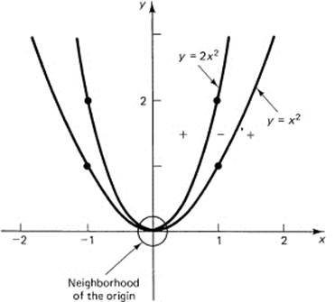
Figure 10.7-1

Thus we see that plausible arguments are not always sufficient. It seems to be so reasonable that: “If for every possible plane section through the z-axis we have a local minimum, then it ought to be a minimum for the function.” Yet it is not. We are not in a position to give a rigorous mathematical proof that the minima we find by least squares are the true minima, but the nature of the surface, quadratic in each parameter, makes one feel relatively safe, even in the face of the above example.

10.8 GENERAL CASE OF LEAST-SQUARES FITTING

An examination of what we have done, using least squares fitting of polynomials, shows that only at few places in the derivation did we depend on the fact that the functions we were using to approximate the data were polynomials. The method depended rather on the fact that the unknown parameters occurred linearly in the formula.

Example 10.8-1

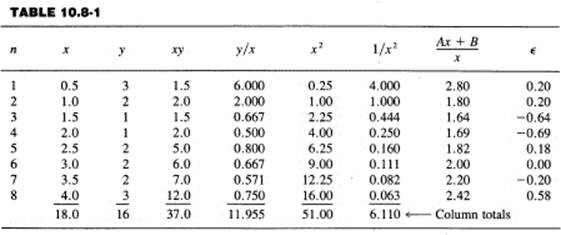
Suppose we want to fit some data by a linear combination of the functions (M = 2) x and 1/x. The original data (N = 8) and the working computations are shown in Table 10.8-1. The numbers are simple, the curve is crude, and normally given noisy data you have at least ten times the number of data points as you have coefficients to be fitted. All of this is neglected to produce an example where you can compute the numbers easily.

We begin with the formula we want:

Suppose we have the curve; then the errors (difference between the given y_n and the value from the fitted line Ax_n + B/x_n) are the residuals,

The principle of least squares says that we should minimize the sum of the squares of these residuals (summed over all the given data); that is, we minimize

To do this, we differentiate with respect to each of the variables (A and B) and set the corresponding derivatives equal to zero.

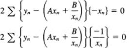
After a slight rearrangement, we get

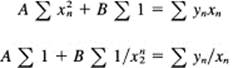
The two coefficients ∑ 1 arise because x(1/x) = 1. From the Table 10.8-1, we have all the coefficients, when we remember that ∑ 1 = 8 in this case because there are eight data points.

These are the normal equations for this problem, and after substituting from the totals of the appropriate columns we have

51A + 8B = 37

8A + 6.11B = 11.955

To eliminate A, multiply the top equation by −8 and the lower by 51 and then add the two equations. As a result we have

B = 1.267 and A = 0.527

We use these to compute the values on the curve as well as the residuals _n in the last column. Figure 10.8-1 shows both the original data and the computed least squares curve. The fit is, of course, crude as you would expect from the crudeness of the data and having only two coefficients to use in fitting the data.

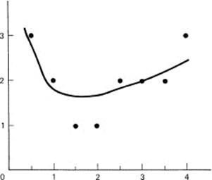
Figure 10.8-1

EXERCISES 10.8

1.Write the normal equations for fitting N data points (x_n, y_n) by three functions u₁(x), u₂(x), and u₃(x).

2.Generalize to fitting the data by M functions u_m(x), m = 1, 2, …, M.

10.9 SUMMARY

The first idea we introduced is that of a function of several variables, and along with this comes the idea of an n-dimensional space. This is the space in which the set of n values are imagined as a point, and the corresponding equations are surfaces (hypersurfaces if you prefer that word). We looked briefly at both linear and quadratic surfaces in three dimensions as natural extensions of what we earlier did in two dimensions. The surfaces studied are useful later.

Then we introduced the central idea of partial derivatives, which are simply derivatives of one variable with respect to another, when all the other variables are held constant. We found that implicit differentiation had a new look in this notation. The general theory of partial differentiation (say in thermodynamics) is very complex, and we have looked only at the simplest parts.

The principle of least squares was introduced, and its virtues (easy to solve such problems) as well as its main fault, too much emphasis on an outlier (error?), were discussed. We fitted a point to a set of data (measured on the same thing) and found that the least squares fit was simply the mean of the values. We then approached fitting straight lines, and later polynomials, to given data, and then finally general functions to sets of data. As long as the coefficients to be determined enter linearly into the formula, and the functions you are combining are linearly independent, then in principle the least squares solution can be found. The emphasis on “in principle” is because when there are many functions the solution may not be well determined, in the sense that small changes in the input numbers will produce large changes in the output (coefficients).

But do not confuse the quality of the least squares fit, which is measured by the sum of the squares of the residuals, with the uncertainty in the coefficients you are determining. It can often happen that the quality of the fit of the curve to the data is good, but that the particular coefficients are ill determined by the data. You merely have a poorly designed experiment if you wanted to determine the coefficients accurately.

The principle of least squares is widely used in many fields to fit data. It is often regarded as “smoothing the data” in some sense, eliminating the “noise of the measurements.” The ease of solution (we are not speaking of the arithmetic labor) makes it very popular. Furthermore, as you will see in later chapters, there is a good deal of theory connected with least squares, and the background of theory gives a better basis for understanding the results than methods that lack the corresponding rich background.