Methods of Mathematics Applied to Calculus, Probability, and Statistics (1985)

Part II. THE CALCULUS OF ALGEBRAIC FUNCTIONS

Chapter 7. Derivatives in Geometry

7.1 A HISTORY OF THE CALCULUS

The calculus is conventionally divided into two parts, the differential and the integral calculus. Historically, the integral calculus arose first, both Euclid and Archimedes having calculated areas and volumes of shapes bounded by other than straight lines and plane surfaces. The differential calculus arose from the problem of finding tangent lines to curves. There are a few early examples of this, but the main development came after the discovery of analytic geometry. So close is the relationship of analytic geometry to the calculus that there is an inevitability to the discovery of the calculus once analytic geometry is generally known (first publicized by Descartes in 1637).

The main development of the calculus came when these two problems, finding areas and finding tangent lines, were recognized as being inverses of each other, which is the fundamental theorem of the calculus. While Isaac Barrow (1630–1677), Newton’s teacher, in a sense knew this theorem, it was the systematic application of the methods, rather than the development of special tricks, that marked the real founding of the calculus by Gottfried Wilhelm von Liebniz (1646–1716), published in 1684, and by Isaac Newton (1642–1727), published in 1687.

From a high art the calculus has been converted to a routine, systematic method, hence its name “calculus.” Over the subsequent years the presentation of the calculus has been polished until it is now easily mastered by the willing student.

7.2 THE IDEA OF A LIMIT

A central idea in the calculus is the limit. Part I has carefully prepared the ground, so it is mainly a matter of reminding the reader of what has already been said with respect to this idea.

We begin with the idea of a limit of a sequence of numbers, indexed by the integer n. For example, consider the sequence {u_n}, where

as n gets larger and larger. Clearly, the sequence approaches the number 0. Indeed, no matter how close to 0 you want me to get (other than a zero distance away), I can find an integer n₀ such that for all larger n the values of u_n are at least that close to 0.

The expressions “as large as you please” and “larger and larger” are conveniently replaced by the words “as n approaches infinity.” This should not be interpreted to mean that the numbers n reach some “number” called “infinity,” but rather to describe colorfully what is going on. Furthermore, we are not saying that the values of the sequence {1/n} reach 0, but only that the numbers in the sequence ultimately get and stay arbitrarily close to 0. There is a big difference between these two statements.

In words, we say that the sequence u_n (in the above particular case u_n = 1/n) approaches a limit, L (which in this case is 0), as n approaches infinity. In symbols we write

For the sequence

the corresponding limit L is clearly 1. The test is that the difference between u_n and its limit L approaches 0.

A sequence that approaches a limit is said to converge to the limit. A sequence that does not converge is said to diverge. For example, the sequence

has values alternately +1 and –1. It does not converge because it never stays close to a limit; rather it continually oscillates between two numbers +1 and –1.

Example 7.2-1

We have already seen (Section 3.6) this idea of convergence several times. When we wrote the decimal digits of the rational number as

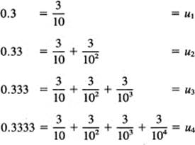
we wrote a sequence of approximations u_n. This, sequence of approximations u_n approaches (and stays close) to the limit . We did not say that any finite number of 3’s was equal to ; we merely said that as we took more and more digits (as the number of digits approached infinity), the sequence of numbers approached the number . We said that was the limit of the sequence.

Example 7.2-2

Another illustration (Example 3.6-4) is the sequence (9/10)ⁿ. We have for the u_n values

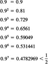
To get a better “feel” for what is happening with respect to the convergence of the sequence, we look for a bound in the more familiar decimal notation. From the last line of numbers (in this example) we see that

and in particular that

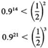
Here we see, in the familiar decimal notation, that the sequence (0.9)ⁿ is approaching 0. Increases in the exponent by 70 multiply the bound by a factor smaller than 1/1000

In Example 3.5-3 we saw how (in principle) we can find a decimal approximation to an algebraic (real) number as accurately as we please. In particular, we constructed a convergent sequence of numbers whose limit was the root of an algebraic equation. As we compute more and more digits of the algebraic number, we approach the root more and more closely.

Sequences that approach zero are called null sequences. They play a central role in the theory. The sequence of differences between a convergent sequence u_n and its limit L is a null sequence. When you study a sum of terms, such as a geometric progression, the series is converted into a sequence of partial sums, and it is the sequence that is tested for convergence. Thus, when we looked at a decimal number, we regarded it as a sum of the individual digits, each digit divided by its corresponding power of 10, and we then studied the sequence of partial sums.

Example 7.2-3

A similar, and more general, example of the above is the geometric progression when the rate r satisfies the inequality of |r| < 1. From Example 2.6-1 we have for the sum of a geometric progression

We first want to show that when |r| < 1 then rⁿ approaches 0. (We just saw this was true when r = 9/10.) If we can show this, then the last term of the sum will approach 0 (will be a null sequence), and the limit of the, sum will be only the first term.

We can prove that the limit of the sequence rⁿ is 0 for any |r| < 1 by using an inequality we derived in Example 3.7-1, that

This a is not to be confused with the a in the geometric progression. To use this inequality, we observe that if |r| < 1 then its reciprocal is greater than 1. Hence there is an a such that

or, in a more convenient form for our immediate need,

Therefore, remembering that the 1 + a is in the denominator, we have the inequality in the reverse direction:

As n approaches infinity, the denominator approaches infinity, and the right-hand side comes as close as you please to 0. You tell me how close you want |r|ⁿ to be to 0 and I can tell you an n such that for all larger indices it is at least that close. I do not need to tell you the smallest n; I only have to tell you one that “works.” We have therefore proved that |r|ⁿ (when |r| < 1) is a null sequence. Hence rⁿ is a null sequence.

Since the rⁿ approaches 0, it follows that the second term in the sum in (7.2-2) of a geometric progression,

must also approach 0 (the term in the brackets is a fixed number independent of n). Thus we say that the S_n (the partial sum) of a geometric progression, as we take more and more terms, approaches the limit S (for |r| < 1), where

and the S_n are the partial sums

of the series. We do not claim that the sum takes on the value of the limit, only that as you let n approach infinity the values of the partial sum ultimately become and stay arbitrarily close to the limit.

This is a good example of a common phenomenon in science. Often, when progress seems to be blocked, the advance is made by evading the question. The question, “Does the sequence reach its limit?” is evaded; we only claim that the sequence gets and stays arbitrarily close to the limit. It turns out that this is good enough for us; we do not need to know more than that.

We have emphasized that to have a limit requires both (1) that the sequence gets close, and (2) past some point the sequence stays close to the limit. Consider the sequence

The limit is 1, and it often takes on that value, and then wanders away, before it finally gets and stays as close as you require. On the other hand, the sequence

does not converge. It does not stay close to either 0 or 1 (or any other number).

Abstraction 7.2-4*

The words we have been using to describe a limit are conventionally expressed in the following mathematical notation (don’t let the Greek letter , lowercase epsilon, bother you). Given any > 0, there exists a number n₀ such that for all integers n ≥ n₀

When we say “any > 0” in a sense we imply “for all numbers > 0,” no matter how large or small. Notice how neatly the mathematics expresses the precise idea of a limit of a sequence.

7.3 RULES FOR USING LIMITS

Example 7.3-1

In using limits we sometimes need to handle complicated expressions. Thus we need to study combinations of limits. From the simple example, as n approaches infinity,

it is easy to see that the limit of a sum is the sum of the limits (provided the individual limits exist). And similarly for differences. Limits of sums and differences are the sums and differences of the limits for any finite number of terms, as you can see, or as you can prove using either ellipsis or mathematical induction.

We next look at products of limits, for example,

Both factors of the product approach 2, and therefore the product approaches 4. To see the details, if you wish to see them, we write the difference between the sequence and its limit as a null sequence:

And as n approaches infinity the right-hand side approaches 0. Therefore,

u_n → 4

as its limit.

Finally, we need to look at quotients. Consider the sequence

The numerator approaches 1 and the denominator approaches 2, so the quotient approaches . If you wish to look at the details, you write the difference as a null sequence

and the first term approaches 0 (when n → ∞) as required (and the other term stays away from 0). If you asked me to find a bound on n beyond which the right-hand side was as close to 0 as some number you required, I would reason as follows. Assuming that n ≥ 2, the denominator of the second term could be replaced by

because this merely makes the right-hand side larger.

Thus I can pick an n such that

which is easily solved for n:

In summary you see that the limits of sums, differences, products, and quotients of limits have the same value as the corresponding combinations of limits (provided the individual limits exist, and in the case of quotients that the denominator limit is not 0).

EXERCISES 7.3

Find the limit as n approaches infinity of the following (assume that the individual coefficients a, b, c, and d are not zero):

1.a + b/n + c/n² + d/n³

2.[a + b/n]/[c + d/n], provided c ≠ 0

3.[a + b/n + c/n³][d + e/n + f/n²]

4.[an + b]/[cn + d], Hint: First divide both numerator and denominator by n.

5.[an³ + 1]/[bn³]

6.[an² + l]/[bn³ – 1]

7.Define a limit.

7.4 LIMITS OF FUNCTIONS—MISSING VALUES

We have looked at limits of sequences; now we turn to limits for continuous functions.

Example 7.4-1

Consider the expression

This is not defined for the value x = 2 since division by 0 is normally excluded. However, for all other values this is equivalent to

y(x) = x + 2

In the original form we are missing one isolated value at x = 2.

Now consider (see Figure 7.4-1) the limit of y(x) as x approaches the value 2, for either larger or smaller values of x. This is simply the value at that point of the equivalent form x + 2. Because of the division by 0, we cannot write

y(2) = 4

for the original form of y(x), but we can write

Read this as: the limit as x approaches 2 of y(x) equals 4.

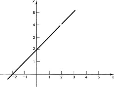
Figure 7.4-1 Missing value at x = 2

The necessity for this circumlocution (circum, around; locutio, to speak) is the desire to avoid the division by zero; most mathematicians simply do not like the thought of dividing by zero. For example, if the unrestricteddivision by 0 were allowed, then from the equation

(0)(3) = (0)(7)

the division by 0 would give

3 = 7

which is a contradiction! In a sense, the limit process can be viewed as a controlled division by zero (a potential as contrasted with an actual zero).

Example 7.4-2

Another example of where we are missing an isolated point in the function (because of an indicated division by 0) is

when x ≠ a. When we consider the limit as x approaches a from either side, we find, on looking at the right-hand side of the equivalent form, that the limit is

a² + a² + a² = 3a²

(merely put x = a in the right-hand side of the above equation).

Example 7.4-3

Consider the trivial example

except for the value x = 0. See Figure 7.4-2. It is natural to take the value at the missing point (x = 0) as the corresponding value of the equivalent form, y = a. Thus, when there is an indicated division by zero, it is often merely a matter of rewriting the expression to eliminate this division to get an equivalent form (equivalent for all values other than the isolated value), and for which the new form gives directly a definite value.

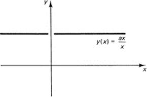
Figure 7.4-2 Missing value at x = 0

This situation, where an isolated value is missing, arises when there is an indicated division by 0 and is of common occurrence. The method of limits handles the problem of determining this missing value. Usually, the value is easy to find, but on occasions it requires some effort. It is a situation, with some variations, that we will often meet.

Example 7.4-4

Consider the function

There is a division by zero to examine. For x > 0 the function is +1, and as x approaches zero from the positive side the limit is +1; but when approached from the negative side the limit is –1 (see Figure 7.4-3). Thus there is no limit as x → 0.

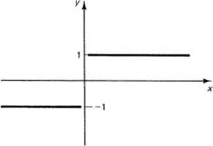
Figure 7.4-3 y = x/|x|

It is an exercise in rereading the limits for sequences to see that for functions the limits of sums, products, and quotients are the corresponding sums, products, and quotients of the limits.

Abstraction 7.4-5*

Corresponding to Abstraction 7.2-4*, we can express the idea of a limit as x → a of a function f(x) as: given any > 0, there exists a δ(Greek lowercase delta) such that for all x in the interval

|x – a| < δ

then

|f(x) – L| >

Notice how this catches the idea in mathematical symbols, which can later be manipulated in mathematical ways; to capture words in the form of symbols is one of the basic processes in doing mathematics.

We can now make the idea of continuity a bit clearer. A function is continuous at a point x = a if both (1) f(a) exists, and (2) lim_x→af(x) = f(a). For continuity at a point x = a, the value of the function at the point must exist, and the limit of the function as you approach the point must be this same value.

Continuity in an interval requires continuity at all points in the interval. This does seem to be close to our intuitive feeling of what we mean by continuity. Using it, we can easily prove that, for example, the powers of x are continuous. Let

y(x) = xⁿ

Then at any point a, f(a) = aⁿ. When we try part (2), we have

The second absolute term value is bounded (near x = a), and the first term approaches zero, so the function is continuous at the point a. Since a was any point along the real line, the powers of x, and hence polynomials, are continuous for any finite interval.

EXERCISES 7.4

Write the following in their equivalent forms and find the corresponding limits.

1.(x² – 2x + 1)/(x² – 3x + 2) as x → 1

2.(x² – 1)/(x – 1) as x → 1

3.(x – 1)/( – 1) as x → 1

4.(x – 1)/( – 1) as x → 1

5.(x – 1)/( – 1) as x → 1

6.(x – aⁿ)/(x – a) as x → a. Hint: See Section 4.7

7. as x → 0. Hint: Multiply numerator and denominator by .

8.Prove that in the interval 1 ≤ x ≤ 2 the function y = is continuous.

7.5 THE Δ PROCESS

We first need to introduce a notation. We will mean by the symbols

Δx

a change in x (Δ is the Greek capital delta). The change may be either positive or negative, although we usually picture it as if Δx were positive. It does not mean a product of Δ times x; it is an operation on x just as sin x means the operation of taking the sine of x. However, it is more general than is the sine function since it is an unspecified amount of change. Sometimes this is written as

Δx = h

Example 7.5-1

Suppose we consider the parabola

y(x) = x²

We have for a given change in x, labeled Δx, the corresponding change in y:

Δy(x) = y(x + Δx) – y(x)

The ratio of the changes is the slope of the line through the points at x and at x + Δx:

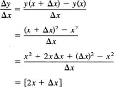
The original expression was not defined for Δx = 0, but we have rewritten the expression in an equivalent form where this isolated point no longer causes trouble. To find the limit as Δx approaches 0, we evaluate the equivalent form, which does not have the awkward division by 0. The result is

2x

Figure 7.5-1 shows the parabola y = x², and the corresponding slopes at selected values of x, such as x = –1, 0, 1, and 2. These limits are the limiting slopes of the secant line of the curve y = x² at the corresponding points. In the limit the secant line becomes the tangent line (by definition).

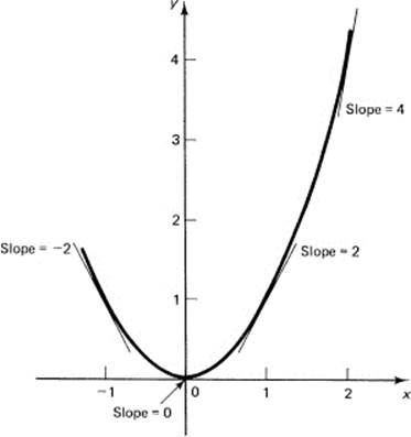
Figure 7.5-1 y = x²

Now consider the general function of x; call it

y = y(x)

Fix the point P = (x, y) in your mind, and then let x be changed, incremented, by the amount Δx; see Figure 7.5-2 for details. The change in x produces a corresponding change in y, called Δy. Thus there are now two points P and Qon the curve of y(x):

P = (x, y) and Q = (x + Δx, y + Δy)

The slope of the secant line through these two points is, of course,

In words, the slope of the secant line is the change in y, called delta y, divided by the change in x, called delta x.

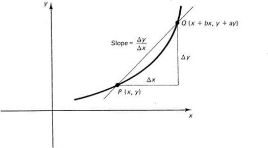
Figure 7.5-2 General slope

We now think of Δx as a variable, and consider the limit of Δy/Δx as Δx approaches 0. We do not let Δx = 0 since that would be a division by 0, but rather, as in Section 7.4, we consider the limit of the quotient as Δx approaches 0. We search for the “missing value,” the limiting slope of the secant line that is the slope of the tangent line.

Geometrically, we have taken the secant line through two nearby points P and Q and then let the point Q approach P. We consider the limiting slope as Δx approaches 0. We see that indeed the limiting slope is the slope of the tangent line to the curve at each point (x, y). In Example 7.5-1 for the parabola y = x², we found that at any point x the slope is 2x.

We need a compact symbol to represent this limiting slope. The suggestive notation due to Leibniz is

Again, the symbol on the right is to be read as a whole, “dee y over dee x,” and not as a quotient. The symbol tells you where it came from, that is, the limit of the quotient of the corresponding deltas.

From the original function

y(x)

we “derived” a new function

It is called “the derivative of y with respect to x.”

Since the derivative plays a dominant role in the differential calculus, we need to describe (give an algorithm for) exactly what we are doing. This is the classic four-step rule. To compute the derivative of a given function y(x), you do the following four steps:

1.Give x an increment Δx.

2.Compute the corresponding change in y:

Δy = y(x + Δx) – y(x)

3.Compute the ratio of the changes:

4.Take the limit as Δx approaches 0.

This last step can be written in the mathematical notation

The four-step rule uses the limit process to handle the division by zero. Stop here and review this rule until you understand exactly how it expresses your ideas of how to find the slope of the tangent line (and hence the local slope of the curve itself).

We turn to some specific examples that are carefully chosen to lead you to more general results. No doubt the first persons did many examples before they saw the general results, and could then avoid the almost endless repetition of the same sort of thing in each special case.

Example 7.5-2

Suppose we try the simple power function

y(x) = x³

Following the four-step rule, we find that from step 3 of the rule we have

As always, some algebra is needed before we try to take the limit. The purpose of the algebra is to eliminate the appearance of the division by the Δx so that the limit is easily found from the equivalent form. In this case we simply expand the binomial and cancel the x³ terms:

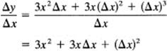
In this equivalent form it is easy to take the limit as Δx approaches 0. The result is

Example 7.5-3

Consider next the function

y(x) = x³ + x

and apply the four-step rule. From the third step we get

We have to rearrange this expression before taking the limit. Expand the binomial and cancel the like terms (both the x³ and the x terms) to get

In this equivalent form we can take the limit without facing a division by zero. We get

Thus the derivative of y(x) = x³ + x is dy/dx = 3x² + 1.

Example 7.5-4

Another example is

The first three steps of the rule produce

Here the rearrangement to remove the division by zero is not so obvious. Some thought (and the first person must have done a lot of thinking) and recalling that

suggests multiplying both numerator and denominator by

This gives, in the numerator, the difference of the squares of the two square roots:

This Δx will now cancel the one in the denominator. The result is

In this form, as Δx approaches zero, we get the limit

Example 7.5-5

Because of the importance of the delta process, we look at a final example:

The third step of the four-step process produces

Again we multiply both numerator and denominator by the sum of the square roots. This time we get the expression

In this form we recognize parts of the last two examples. The first [ ] is the immediately preceding, Example 7.5-4, with x³ + x in place of x, and the second [ ] is exactly Example 7.5-3. The limit is, therefore, the product of the limits (Section 7.3)

The four-step delta process involves in step 3 a division by Δx and then in step 4 the limiting process as Δx → 0. The limiting process requires that you first rearrange the difference quotient Δy/Δx into an equivalent form so that the limit can be found. This uses the methods of Section 7.4, so we can find the “missing value.” We say that the slope of the curve at the given point is the slope of the tangent line at that point.

EXERCISES 7.5

Apply the four-step delta process to the following:

1.y = x⁴

2.y = ax² + bx + c

3.y = 1/x

4.y = 1/(x + 1)

5.y = + 1

6.y = 5x⁴

7.y =

8.y = 1/(x² + 1)

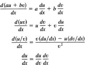
7.6 COMPOSITE FUNCTIONS

The last three examples show why we want to think about the composition of functions, such as

which is composed of the function “sine” of the function “square root” of x. Such a function is called a composite function. We saw in Example 7.5-5 that the delta process effectively took the derivative of the first function and multiplied this by the derivative of the second function.

To fix notation, suppose we have a pair of functions y and u, such that

y(x) = y[u(x)]

much like the above example, where we had y = and u = x³ + x. It is immediately obvious that (for Δx and Δu both not 0)

and if the separate limits exist, then in the limit we have the fundamental relationship

This is the important composite function rule, also sometimes called the chain rule.

Example 7.6-1

In Example 7.5-5, we had

We think of and u = x³ + x. From Example 7.5-4, we found that if

then

and from Example 7.5-3 we found that if

u(x) = x³ + x

then du/dx is given by

Therefore, we conclude from Equation (7.6-1) that in this example

which is what we got before (Example 7.5-5).

Thus if we know how to find the derivatives of simple functions, it is easy to pass via the composite function rule (7.6-1) to more complex functions. Indeed, the composite rule for functions of functions of functions, and so on, is clearly

and we can go as deep in the notation as we please. We need to turn, therefore, to finding the derivative of simple functions of some generality.

In the spirit of generalization consider, next, the general integral power of x

y(x) = cxⁿ

From step 3 of the four-step rule, we have (factoring out the c)

One way of making further progress is to recall the algebraic identity (Section 4.7), or simply multiply out the right-hand side and note the cancellation:

Then apply this to the difference of the two nth powers, where b = x + Δx and a = x. It works out nicely because

and the difference quotient is merely the second parentheses of the algebraic identity. The final step is to take the limit as Δx approaches 0. Looking at the equivalent expression,

we see that each term in the brackets will approach

x^n-1

and that there are exactly n such terms. Therefore, the derivative of cxⁿ is

This is a fundamental rule of the differential calculus. Notice that you “pass over” the constant c in front of the expression and differentiate xⁿ. When you follow the algebra, you see that as a general rule the constant c factors out of each term and enters into the derivation at each step only as a front constant.

An alternative derivation can be based on expanding the binomial (x + Δx)ⁿ, canceling the xⁿ term, dividing by Δx, and then taking the limit. All the terms of the expansion except the first one that is left will approach zero and you will have the same result.

Example 7.6-2

If

y = 3x¹⁷

then the derivative is

The special case of n = 0 requires separate investigation. The exponent equal to zero means that the function cx⁰ is a constant,

y(x) = c

Just considering what this function is, a horizontal line, and the meaning of the derivative in geometry, that is, the local slope at the point x, shows that the derivative must be zero. However, we will go through the basic four-step process. Remember y(x) = c for all x. At step 2 of the four-step process, we have

Divide by Δx to get at step 3

This is always zero (for Δx ≠ 0), so the limit in step 4 is also zero. Thus we have the rule that the derivative of a constant is 0.

Differentiation is a fundamental process that must be mastered so well that it is almost automatic. The student is apt to think that the formulas can always be looked up when needed. But consider the situation where you are teaching a child the multiplication tables. The child says, “Why must I learn them perfectly, I can always look them up or use a hand computer?” The answer is, of course, there will come a time when the child faces division and needs to know the multiplication table so well that the number 21 immediately calls up to mind 3 times 7. Indeed, when it comes to factoring polynomials and the number 12 arises, then all combinations must be already in mind.

so that the factoring of

can be done reasonably efficiently; the algebraic sum of the two factors must be the “something.”

So it is with the process of differentiation. Not only must you be able to go directly from the functions to their derivatives, but there will soon come a time when the problem is to go in the reverse direction; from the given derivative you must be able to answer rapidly and reliably the question, “Where did this derivative come from?” You must be able, almost instantly, to imagine a large number of possibilities. Therefore, you are urged to learn the process of differentiation, at each stage, so well that you can do it reliably and almost without thought.

At the moment we have two basic general rules (including the case n = 0, a constant):

and

You can see them working together in the simple example

x^mn = (xⁿ)^m

Differentiate both sides in their respective forms (use u = xⁿ on the right-hand side) to get

which after a little algebra is

and is obviously true. You can mentally practice differentiation at odd moments using special cases of the identity

(x^m)ⁿ = x^mn

EXERCISES 7.6

Differentiate on sight:

1.1, x, x², x³, x⁴, x¹⁹, x¹, xⁿ

2.6x², 4x³, 3x⁴, 2x⁶, x¹²

3.ax¹, cx³, bxⁿ, 6, 3ax⁴

Apply the delta process to the following:

4.x⁴

5.7x³

6.17x²

7.Show in detail that the derivatives of x²¹ and (x⁷)³ are the same.

8.Derive the rule for differentiating xⁿ using the binomial theorem.

7.7 SUMS OF POWERS OF X

Now that we can differentiate individual positive powers of x we turn to the examination of sums of powers of x. As a first, simple example (note the use of prime numbers so you can follow the way things go), consider the following example.

Example 7.7-1

If

We get for step 2 of the four-step rule

so that at step 3 (expand the first term by the binomial theorem, cancel like terms, and divide by Δx)

Therefore, doing step 4 we get

The result is the same as if we passed over the constant coefficients and differentiated each power of x term by term.

It is easy to generalize to the sum of two (or more) functions. Suppose we have two functions u(x) and v(x) and that

Now thinking about how the algebra in Example 7.7-1 went, we see that we can group the terms in a and b separately. Thus we are led to the corresponding expressions (at step 3)

and in the limit we will have

It is evident (using mathematical induction) that the rule applies to any finite sum of terms. The rule for differentiating any finite sum of terms is: differentiate term by term and pass over (but copy down) any constants that may occur in front of the powers of x. In words, differentiation is a linear operation; the derivative of a sum is the sum of the derivatives. Remember that the derivative of a constant is 0.

Example 7.7-2

Given the function

the derivative can be written down immediately (using 7.7-1) as

Example 7.7-3

Another example of more general form (we are deliberately forcing generality on you) is the general polynomial

The derivative is, upon inspection,

Example 7.7-4

As an example of a composite function, consider

We say to ourselves, we have some function u(x) to the seventh power; therefore,

where u(x) = x³ + x + 11, and of course, from (7.7-1),

Therefore,

Example 7.7-5

A more complex example is

Take it term by term. The first term is a seventh power of something. Reason as follows: the derivative is 7[something] to the sixth power times the derivative of what is inside and that is (looking at the 5x² + 1) exactly 10x. So the first term gives

7[5x² + 1]⁶(10x)

Apply the same technique to each term, thus getting, finally,

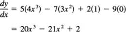
after a little algebra.

This last example shows that after the process of formal differentiation there is often a large amount of what appears to be trivial algebra to get the final result into a decent form. There is a tendency to ignore the importance of this step, but if it is not done correctly, all the earlier work is wasted. Thus a course in the calculus consists to a great extent in learning to do algebra rapidly and reliably, a fact of life that also assures you that you will always be able to do algebra in the future.

EXERCISES 7.7

Differentiate on sight the following:

1.x² + a²

2.x³ – 3x²

3.x³ + x² + x + 1

4.4x² – 2x + 1

5.x³/3 + x²/2 + 1

6.ax² + bx + c

7.axⁿ + bx^m

8.(a + 1)xⁿ

9.xⁿ – aⁿ

Differentiate the following:

10.3(x² + 1)³ + 4(x² – 1)²

11.(a² + x²)ⁿ + (a² – x²)^m

12.(x + 1)³ + 3(x + 1)² + 7

7.8 PRODUCTS AND QUOTIENTS

Suppose you have a product of two functions, say

or in general

What is the derivative? We apply the basic four-step rule: in step 1, first x gets an increment Δx; then, step 2, this induces increments in u to u + Δu, v to v + Δv, as well as in y to y + Δy; next, step 3, we take the ratio to get

Expand the product and rearrange the terms to get

In the last step (4), the limits of these terms, as Δx approaches 0, are

In words, the derivative of a product is the first times the derivative of the second plus the second times the derivative of the first. Don’t learn it in terms of u and v because in use you will be thinking about terms that may have any letters. Note the symmetry in the formula. Since uv = vu (multiplication is commutative), the formula must be symmetric in u and v.

Example 7.8-1

In the example at the beginning of this section,

we have

Therefore, applying the formula for the product, we get

Usually, there are common powers that can be factored out; each common factor is of one lower power than in the original formula. The result is

Example 7.8-2

Find the derivative of

Apply the formula for the product to get

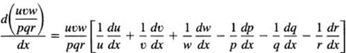
Naturally, products of three or more terms can occur, and we need to look at extensions of the formula. Consider the formula

y = uvw

We can look at this as either of the forms

y = (uv)w = u(uw)

and apply the product rule. In the first case we have

and to the last term we again apply the product rule

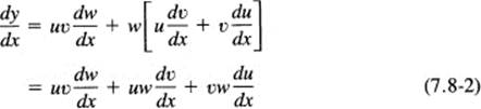
Again note the necessary symmetry. Indeed, you can now easily see (and prove by induction if you wish) the formula for the product of any number of terms. The derivative of a product of n terms is the sum of n distinct terms in each of which only one factor is differentiated and all the others are copied as given. No products of derivatives occur.

For a quotient of two functions, we proceed in a similar manner as we did for the product. Suppose

Apply the four-step rule. At step 3 you will have

Get a common denominator

and then rearrange in the form

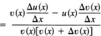
Taking the limit, we have the formula for a quotient:

In words, the derivative of a quotient is the denominator times the derivative of the numerator minus the numerator times the derivative of the denominator, all divided by the denominator squared.

In all these derivations there are many terms that are present before the limit is taken, and which vanish in the limit. Thus the mathematics of the limiting form is generally much simpler than is the finite form before the limit is taken. This is one reason why the algebra and other mathematics for the calculus is much simpler than is the corresponding discrete mathematics.

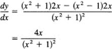
Example 7.8-3

Differentiate

Applying the formula for the quotient, we get

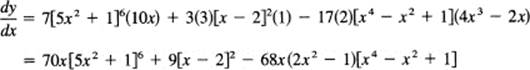
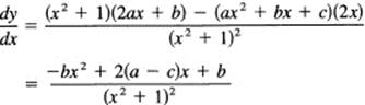
Example 7.8-4

Differentiate

Using the quotient formula, we get

EXERCISES 7.8

Differentiate both sides to check your work.

1.(x – 1)(x + 1) = (x² – 1)

2.(x² – 1)(x² + 1) = x⁴ −1

3.(x² + 1)² = (x² + 1)(x² + 1)

4.(x² – 1)/(x – 1) = x + 1

5.(x + 1)(x + 2)(x + 3) = x³ + 6x² + 11x + 6

Differentiate the following:

6.(x² + a²)(x2 + b²)

7.(x² – a²)(x² – b²)(x² – c²)

8.(x + 1)/(x + 1)

9.x/(x – a)

10.(x + a)/(x + b)

11.(x³ + a³)/(x² + a²)

12.(a²x² + b⁴)/(a²x² – b⁴)

13.Apply the product formula to xⁿ = xxx … x

14.Apply the product rule to xⁿx^m = x^m+n

15.Apply the quotient rule to x^m/xⁿ = x^m–n

7.9 AN ABSTRACTION OF DIFFERENTIATION

Rather than going back again and again to the basic four-step delta process, let us examine just how little we need to have so we can find the derivative of any algebraic function. What rules of differentiation suffice to generate all the rest of the rules for algebraic differentiation?

Clearly, we need both the sum formula,

and the product formula,

Both are easily extended to many terms by recognizing that the product of any two terms may be regarded as a single function. We also need the important function of a function formula:

It turns out (by trial and error) that we also need two more derivatives

and

both of which are easy. From these five formulas alone we will derive all the others using the methods of extension you have already learned.

First, note that applying the product formula to an expression of the form cu (x) gives the rule that you pass over constants.

We next use the model of the laws of exponents (Section 3.8). We write simply

x² = xx

and differentiate both sides [on the right using the product formula (7.9-2) and (7.9-4)]:

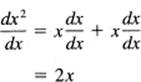
We see the basis for an induction proof (Section 2.3). Assume that the formula

holds up to n = m – 1. Now take the mth case,

x^m = xx^m–1

and differentiate both sides:

The induction is complete for positive integer powers.

Next, to extend the rule to negative powers, we write

1 = xⁿx^-n

and differentiate both sides [using the product formula (7.9-2)] to get

Solve for

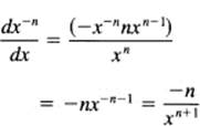
This is the same formula as for positive powers of x; you decrease the exponent by 1.

To attack the fractional powers, we begin by writing

and differentiate both sides (again using the product formula). We get

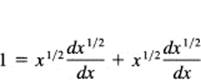
Solve for the derivative:

Evidently, we can similarly find that for the qth root

We are supposing that at this point you can supply the necessary ellipsis proof. Now we have only to use the pth power of the qth root to get the derivative of x^p/q. We have, using the function of a function formula (7.9-3),

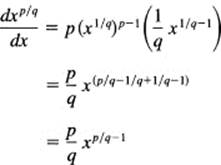
Thus we see that, using a somewhat standard pattern for the extension of ideas, we have found the derivative for all rational powers of the variable x [and by the function of function formula (7.9-3) this applies to rational powers of anything at all]. For the irrational powers such as

we have to appeal, at this point, to the continuity of x′ as a function of n and the assumption that, if the formula holds for the everywhere dense rationals, then it also holds true for the irrationals (see Section 4.5 where this assumption 1 is explicitly stated).

We have finally to derive (again) the formula for the derivative of the quotient of two functions. We write the quotient as a product

Then, applying the product formula (7.9-2),

We get a common denominator and have

Thus we have found all the formulas we need for the moment using only five basic ones. These basic formulas used the four-step rule; the others followed logically from them.

EXERCISES 7.9

Differentiate the following:

1.1/x, 1/x², x⁻³, 5x⁻⁵

2.1/(a + x)

3.1/(a² + x²)

4.1/(a² + x²)²

5.1/(a² − x²)²

6.

7.2x^1/2, (2x)^1/2

8.3x^2/3

9.x^−1/2

10.3x^−1/3

11.

12.(b − x)^−1/2

13.

14.1/

15.x/(a² − x²)

16. + 1/

17.

18.

19.x^4/3 + x^−4/3

20.( − 1)/( + 1)

21.[( − 1)/( + 1)]^1/2

7.10 ON THE FORMAL DIFFERENTIATION OF FUNCTIONS

Just how should you approach a formula when it is to be differentiated? If it is a sum, you use the divide and conquer rule; take the terms one at a time (and try not to get lost when you finish one term but remember to go on to the next term of the sum). For example,

You take one term of the sum at a time. This way the sum is broken down to a number of simpler problems. The first term goes easily, simply

63x⁸

The second term is a product, the first times ….

Now we look at this and see (again!) the simple differentiations of sums:

We have to assemble the parts of the derivatives of the first two terms. Then we remember that there is a third term. This is a quotient and we start, denominator times ….

We need to assemble the results of the three terms

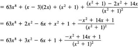
Thus the process of formal differentiation is broken down to a sequence of simpler differentiations. When you begin, it is wise to write out the steps one at a time so that you do not get lost. In effect, you are trying to push the derivative sign off the right-hand side of the expression, and you finally get rid of it when you have a derivative of x with respect to x (you simply pass over constants in front of terms). You are done when there are no more derivatives to be taken. But the differentiation process is laborious, and gradually you begin to keep a mental “pushdown list” of where you are, and you start eliminating the writing down of many of the trivial steps. Of course, there is often a lot of final algebra to be done to clean up the mess that appears on the paper.

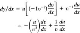
There is not a unique, single way of attacking a differentiation problem. For example, suppose you have a problem in the form

You can look at it in many ways. Among others are

They must all give the same result. In the first case, (u/w)v, you have

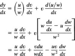
In the second case, u(v/w), you get

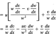
which is the same thing with a different order of terms.

If the equations are written in the form with the original function factored out in front, then you have

From this you can make a good guess that the general case is

where there is a plus sign in front of the terms in the numerator and minus signs in front of the denominator terms.

Formal differentiation is a necessary process to master. We will use it constantly throughout the rest of the book. It is a matter of practice until it is almost automatic and you can concentrate on the use you are going to make of the derivative when you get it. Blind practice is not as effective as intelligent practice, especially going over a completed problem to see why and how things went, criticizing your attack, and trying the same problem another way until you understand “the way things go.” You need to develop a suitable technique for this important process. From each particular case you should try to understand how other similar cases would go. You can make up as many drill problems as you think you need and check yourself by computing the derivative in two or more ways; problems that you make yourself are apt to be more effective learning experiences than those from a textbook!

EXERCISES 7.10

Differentiate the following:

1.x^1/3 + 2x^2/3 + 3x^4/3

2.(ax² + bx + c)/(x² − 1)

3.p^m(1 − p)^n−m, where the variables is p

4.x(x − 1)(x − 2)(x − 3)

5.1/x(x + 1)

6.1/

7.1/x^4/3

8.−x^−1/5

9.(x − a)(x − b)/(x − c)

10.1/x^−1/2

7.11 SUMMARY

From a formal point of view, differentiation is the basic operation of the calculus. Fundamentally, it is the four-step rule whose meaning, geometrically, is finding the slope of the local tangent line to the curve. From this rule a number of basic rules were derived, which save you from going back to all the details of the four-step rule. We found that

for all real n, not just the integers. Other rules are

Using these five simple rules, you can differentiate any algebraic function. This process of formal differentiation should be mastered so well that whenever you need to differentiate a function you can do so without having to think very much (and thus distract yourself from the new material at hand). We repeat this important point: voluminous practice is not as effective as a reasonable amount done thoughtfully; especially when you finish an exercise, ask yourself what other kinds could be done essentially the same way. Looking back at successes is an efficient way of mastering the tedious art of differentiation. Many short sessions are generally more effective than a few long ones.

You should not forget, while doing the formal differentiation, that the derivative is actually defined by the four-step rule, and the rules you use come from it. All the derivatives you find can be found, in principle, by the direct application of the four-step rule, but to carry out the delta process in full detail would often defeat all your energy. Thus, although at first they are troublesome to master, the simple rules for differentiation represent an enormous saving of effort.

MISCELLANEOUS EXERCISES

Find the derivatives for the following:

1.y = (x² + 1)(x² − 1)

2.y = x/(x + 1)

3.y = x/(1 − x²)

4.y = (x⁴ − 1)/(x + 1)

5.y = [(1 − s)/(1 + s)]^1/2

6.y = (x^1/2 + a^1/2)

7.y = x² + x(x + 1)

8.y = u² + 1, u = v² − 1, v = x² + 1

9.y = (x² + a²)/(x² − a²)

10.y = x² +

11.s = t²/(a² − t²)

12.y = (1 − )³

13.y = [a^2/3 − x^2/3]^3/2

14.y = [1 + {1 + (1 + x²)²}²]²

15.y = x

16.y =

17.y = (x + 1)/(x − 1) + (x − 1)/(x + 1)

18.y = 1/(x)

19.y = x² + 3ax − a²

20.y =

21.y =

22.y = (x² + a²)^3/2

23.s = t²(1 − t)³

24.

25.x = 1/{y²(y + a)²}