Mathematics, Substance and Surmise: Views on the Meaning and Ontology of Mathematics (2015)

Experimental computation as an ontological game changer: The impact of modern mathematical computation tools on the ontology of mathematics

David H. Bailey¹ and Jonathan M. Borwein²

(1)

Lawrence Berkeley National Laboratory (retired), Berkeley, CA 94720, USA

(2)

CARMA, The University of Newcastle, University Drive, Callaghanm, NSW, 2308, Australia

David H. Bailey (Corresponding author)

Email: david@davidhbailey.com

Jonathan M. Borwein

Email: Jonathan.Borwein@newcastle.edu.au

Abstract

Robust, concrete and abstract, mathematical computation and inference on the scale now becoming possible should change the discourse about many matters mathematical. These include: what mathematics is, how we know something, how we persuade each other, what suffices as a proof, the infinite, mathematical discovery or invention, and other such issues.

1 Introduction

Like almost every other field of fundamental scientific research, mathematics (both pure and applied) has been significantly changed by the advent of advanced computer and related communication technology. Many pure mathematicians routinely employ symbolic computing tools, notably the commercial products Maple and Mathematica, in a manner that has become known as experimental mathematics: using the computer as a “laboratory” to perform exploratory experiments, to gain insight and intuition, to discover patterns that suggest provable mathematical facts, to test and/or falsify conjectures, and to numerically confirm analytically derived results.

Applied mathematicians have adopted computation with even more relish, in applications ranging from mathematical physics to engineering, biology, chemistry, and medicine. Indeed, at this point it is hard to imagine a study in applied mathematics that does not include some computational content. While we should distinguish “production” code from code used in the course of research, the methodology used by applied mathematics is essentially the same as the experimental approach in pure mathematics: using the computer as a “laboratory” in much the same way as a physicist, chemist, or biologist uses laboratory equipment (ranging from a simple test tube experiment to a large-scale analysis of the cosmic microwave background) to probe nature [51, 53].

This essay addresses how the emergence and proliferation of experimental methods has altered the doing of mathematical research, and how it raises new and often perplexing questions of what exactly is mathematical truth in the computer age. Following this introduction, the essay is divided into four sections¹: (i) experimental methods in pure mathematics, (ii) experimental methods in applied mathematics, (iii) additional examples (involving a somewhat higher level of sophistication), and (iv) concluding remarks.

2 The experimental paradigm in pure mathematics

By experimental mathematics we mean the following computationally-assisted approach to mathematical research [24]:

1.

Gain insight and intuition;

2.

Visualize mathematical principles;

3.

Discover new relationships;

4.

Test and especially falsify conjectures;

5.

Explore a possible result to see if it merits formal proof;

6.

Suggest approaches for formal proof;

7.

Replace lengthy hand derivations;

8.

Confirm analytically derived results.

We often call this ‘experimental mathodology.’ As noted in [24, Ch. 1], some of these steps, such as to gain insight and intuition, have been part of traditional mathematics; indeed, experimentation need not involve computers, although nowadays almost all do. In [20–22], a more precise meaning is attached to each of these items. In [20, 21] the focus is on pedagogy, while [22] addresses many of the philosophical issues more directly. We will revisit these items as we continue our essay. With regards to item 5, we have often found the computer-based tools useful to tentatively confirm preliminary lemmas; then we can proceed fairly safely to see where they lead. If, at the end of the day, this line of reasoning has not led to anything of significance, at least we have not expended large amounts of time attempting to formally prove these lemmas (for example, see Section 2.6).

With regards to item 6, our intending meaning here is more along the lines of “computer-assisted” or “computer-directed proof,” and thus is distinct from methods of computer-based formal proof. On the other hand, such methods have been pursued with significant success lately, such as in Thomas Hales’ proof of the Kepler conjecture [36], a topic that we will revisit in Section 2.10. With regards to item 2, when the authors were undergraduates they both were taught to use calculus as a way of making accurate graphs. Today, good graphics tools (item 2) exchanges the cart and the horse. We graph to see structure that we then analyze [20, 21].

Before turning to concrete examples, we first mention two of our favorite tools. They both are essential to the attempts to find patterns, to develop insight, and to efficiently falsify errant conjectures (see items 1, 2, and 4 in the list above).

Integer relation detection. Given a vector of real or complex numbers x _i , an integer relation algorithm attempts to find a nontrivial set of integers a _i , such that . One common application of such an algorithm is to find new identities involving computed numeric constants.

For example, suppose one suspects that an integral (or any other numerical value) x ₁ might be a linear sum of a list of terms . One can compute the integral and all the terms to high precision, typically several hundred digits, then provide the vector (x ₁, x ₂, …, x _n ) to an integer relation algorithm. It will either determine that there is an integer-linear relation among these values, or provide a lower bound on the Euclidean norm of any integer relation vector (a _i ) that the input vector might satisfy. If the algorithm does produce a relation, then solving it for x ₁ produces an experimental identity for the original integral. The most commonly employed integer relation algorithm is the “PSLQ” algorithm of mathematician-sculptor Helaman Ferguson [24, pp. 230–234], although the Lenstra-Lenstra-Lovasz (LLL) algorithm can also be adapted for this purpose. In 2000, integer relation methods were named one of the top ten algorithms of the twentieth century by Computing in Science and Engineering. In our experience, the rapid falsification of hoped-for conjectures (item #4) is central to the use of integer relation methods.

High-precision arithmetic. One fundamental issue that arises in discussions of “truth” in mathematical computation, pure or applied, is the question of whether the results are numerically reliable, i.e., whether the precision of the underlying floating-point computation was sufficient. Most work in scientific or engineering computing relies on either 32-bit IEEE floating-point arithmetic (roughly seven decimal digit precision) or 64-bit IEEE floating-point arithmetic (roughly 16 decimal digit precision). But for an increasing body of studies, even 16-digit arithmetic is not sufficient. The most common form of high-precision arithmetic is “double-double” (equivalent to roughly 31-digit arithmetic) or “quad-precision” (equivalent to roughly 62-digit precision). Other studies require very high precision—hundreds or thousands of digits.

A premier example of the need for very high precision is the application of integer relation methods. It is easy to show that if one wishes to recover an n-long integer relation whose coefficients have maximum size d digits, then both the input data and the integer relation algorithm must be computed using at somewhat more than nd-digit precision, or else the underlying relation will be lost in a sea of numerical noise.

Algorithms for performing arithmetic and evaluating common transcendental functions with high-precision data structures have been known for some time, although challenges remain. Computer algebra software packages such as Maple and Mathematica typically include facilities for arbitrarily high precision, but for some applications researchers rely on internet-available software, such as the GNU multiprecision package. In many cases the implementation and high-level auxiliary tools provided in commercial packages are more than sufficient and easy to use, but ‘caveat emptor’ is always advisable.

2.1 Digital integrity, I

With regards to #8 above, we have found computer software to be particularly effective in ensuring the integrity of published mathematics. For example, we frequently check and correct identities in mathematical manuscripts by computing particular values on the left-hand side and right-hand side to high precision and comparing results—and then, if necessary, use software to repair defects—often in semi-automated fashion. As authors, we often know what sort of mistakes are most likely, so that is what we hunt for.

As a first example, in a study of “character sums” we wished to use the following result derived in [28]:

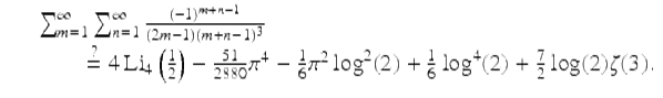
(1)

Here Li₄(1∕2) is a 4-th order polylogarithmic value. However, a subsequent computation to check results disclosed that whereas the left-hand side evaluates to , the right-hand side evaluates to . Puzzled, we computed the sum, as well as each of the terms on the right-hand side (sans their coefficients), to 500-digit precision, then applied the PSLQ algorithm. PSLQ quickly found the following:

(2)

In other words, in the process of transcribing (1) into the original manuscript, “151” had become “51.” It is quite possible that this error would have gone undetected and uncorrected had we not been able to computationally check and correct such results. This may not always matter, but it can be crucial.

Along this line, Alexander Kaiser and the present authors [13] have developed some prototype software to refine and automate this process. Such semi-automated integrity checking becomes pressing when verifiable output from a symbolic manipulation might be the length of a Salinger novel. For instance, recently while studying expected radii of points in a hypercube [26], it was necessary to show existence of a “closed form” for

(3)

The computer verification of [26, Thm. 5.1] quickly returned a 100, 000-character “answer” that could be numerically validated very rapidly to hundreds of places (items #7 and #8). A highly interactive process reduced a basic instance of this expression to the concise formula:

(4)

where Cl₂ is the Clausen function (Cl₂ is the simplest non-elementary Fourier series). Automating such reductions will require a sophisticated simplification scheme with a very large and extensible knowledge base, but the tool described in [13] provides a reasonable first approximation. At this juncture, the choice of software is critical for such a tool. In retrospect, our Mathematica implementation would have been easier in Maple, due to its more flexible facility for manipulating expressions, while Macsyma would have been a fine choice were it still broadly accessible.

2.2 Discovering a truth

Giaquinto’s [32, p. 50] attractive encapsulation

In short, discovering a truth is coming to believe it in an independent, reliable, and rational way.

has the satisfactory consequence that a student can legitimately discover things already “known” to the teacher. Nor is it necessary to demand that each dissertation be absolutely original—only that it be independently discovered. For instance, a differential equation thesis is no less meritorious if the main results are subsequently found to have been accepted, unbeknown to the student, in a control theory journal a month earlier—provided they were independently discovered. Near-simultaneous independent discovery has occurred frequently in science, and such instances are likely to occur more and more frequently as the earth’s “new nervous system” (Hillary Clinton’s term in a policy address while Secretary of State) continues to pervade research.

Despite the conventional identification of mathematics with deductive reasoning, in his 1951 Gibbs lecture, Kurt Gödel (1906–1978) said:

If mathematics describes an objective world just like physics, there is no reason why inductive methods should not be applied in mathematics just the same as in physics.

He held this view until the end of his life despite—or perhaps because of—the epochal deductive achievement of his incompleteness results.

Also, we emphasize that many great mathematicians from Archimedes and Galileo—who reputedly said “All truths are easy to understand once they are discovered; the point is to discover them.”—to Gauss, Poincaré, and Carleson have emphasized how much it helps to “know” the answer beforehand. Two millennia ago, Archimedes wrote, in the Introduction to his long-lost and recently reconstituted Method manuscript,

For it is easier to supply the proof when we have previously acquired, by the method, some knowledge of the questions than it is to find it without any previous knowledge.

Archimedes’ Method can be thought of as a precursor to today’s interactive geometry software, with the caveat that, for example, Cinderella, as opposed to Geometer’s SketchPad, actually does provide proof certificates for much of Euclidean geometry.

As 2006 Abel Prize winner Lennart Carleson describes, in his 1966 speech to the International Congress on Mathematicians on the positive resolution of Luzin’s 1913 conjecture (namely, that the Fourier series of square-summable functions converge pointwise a.e. to the function), after many years of seeking a counterexample, he finally decided none could exist. He expressed the importance of this confidence as follows:

The most important aspect in solving a mathematical problem is the conviction of what is the true result. Then it took 2 or 3 years using the techniques that had been developed during the past 20 years or so.

In similar fashion, Ben Green and Terry Tao have commented that their proof of the existence of arbitrarily long sequence of primes in arithmetic progression was undertaken only after extensive computational evidence (experimental data) had been amassed by others [24]. Thus, we see in play the growing role that intelligent large-scale computing can play in providing the needed confidence to attempt a proof of a hard result (see item 4 at the start of Section 2).

2.3 Digital assistance

By digital assistance, we mean the use of:

1.

Integrated mathematical software such as Maple and Mathematica, or indeed MATLAB and their open source variants such as SAGE and Octave.

2.

Specialized packages such as CPLEX (optimization), PARI (computer algebra), SnapPea (topology), OpenFoam (fluid dynamics), Cinderella (geometry), and MAGMA (algebra and number theory).

3.

General-purpose programming languages such as Python, C, C, and Fortran-2000.

4.

Internet-based applications such as: Sloane’s Encyclopedia of Integer Sequences, the Inverse Symbolic Calculator,² Fractal Explorer, Jeff Weeks’ Topological Games, or Euclid in Java.

5.

Internet databases and facilities including Excel (and its competitors) Google, MathSciNet, arXiv, Wikipedia, Wolfram Alpha, MathWorld, MacTutor, Amazon, Kindle, GitHub, iPython, IBM’s Watson, and many more that are not always so viewed.

A cross-section of Internet-based mathematical resources is available at http://www.experimentalmath.info. We are of the opinion that it is often more realistic to try to adapt resources being built for other purposes by much-deeper pockets, than to try to build better tools from better first principles without adequate money or personnel.

Many of the above tools entail data-mining in various forms, and, indeed, data-mining facilities can broadly enhance the research enterprise. The capacity to consult the Oxford dictionary and Wikipedia instantly within Kindle dramatically changes the nature of the reading process. Franklin [31] argues that Steinle’s “exploratory experimentation” facilitated by “widening technology” and “wide instrumentation,” as routinely done in fields such as pharmacology, astrophysics, medicine, and biotechnology, is leading to a reassessment of what legitimates experiment. In particular, a “local theory” (i.e., a specific model of the phenomenon being investigated) is not now a prerequisite. Thus, a pharmaceutical company can rapidly examine and discard tens of thousands of potentially active agents, and then focus resources on the ones that survive, rather than needing to determine in advance which are likely to work well. Similarly, aeronautical engineers can, by means of computer simulations, discard thousands of potential designs, and submit only the best prospects to full-fledged development and testing.

Hendrik Sørenson [49] concisely asserts that experimental mathematics—as defined above—is following a similar trajectory, with software such as Mathematica, Maple, and MATLAB playing the role of wide instrumentation:

These aspects of exploratory experimentation and wide instrumentation originate from the philosophy of (natural) science and have not been much developed in the context of experimental mathematics. However, I claim that e.g. the importance of wide instrumentation for an exploratory approach to experiments that includes concept formation also pertain to mathematics.

In consequence, boundaries between mathematics and the natural sciences, and between inductive and deductive reasoning are blurred and becoming more so (see also [4]). This convergence also promises some relief from the frustration many mathematicians experience when attempting to describe their proposed methodology on grant applications to the satisfaction of traditional hard scientists. We leave unanswered the philosophically-vexing if mathematically-minor question as to whether genuine mathematical experiments (as discussed in [24]) truly exist, even if one embraces a fully idealist notion of mathematical existence. It surely seems to the two of us that they do.

2.4 Pi, partitions, and primes

The present authors cannot now imagine doing mathematics without a computer nearby. For example, characteristic and minimal polynomials, which were entirely abstract for us as students, now are members of a rapidly growing box of concrete symbolic tools. One’s eyes may glaze over trying to determine structure in an infinite family of matrices including

but a command-line instruction in a computer algebra system will reveal that both and thus illustrating items 1 and 3 at the start of Section 2. Likewise, more and more matrix manipulations are profitably, even necessarily, viewed graphically. As is now well known in numerical linear algebra, graphical tools are essential when trying to discern qualitative information such as the block structure of very large matrices, thus illustrating item 2 at the start of Section 2. See, for instance, Figure 1.

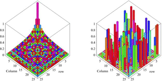
Fig. 1

Plots of a 25 × 25 Hilbert matrix (L) and a matrix with 50% sparsity and random [0, 1] entries (R).

Equally accessible are many matrix decompositions, the use of Groebner bases, Risch’s decision algorithm (to decide when an elementary function has an elementary indefinite integral), graph and group catalogues, and others. Many algorithmic components of a computer algebra system are today extraordinarily effective compared with two decades ago, when they were more like toys. This is equally true of extreme-precision calculation—a prerequisite for much of our own work [19, 23–25]. As we will illustrate, during the three decades that we have seriously tried to integrate computational experiments into research, we have experienced at least twelve Moore’s law doublings of computer power and memory capacity, which when combined with the utilization of highly parallel clusters (with thousands of processing cores) and fiber-optic networking, has resulted in six to seven orders of magnitude speedup for many operations.

2.5 The partition function

Consider the number of additive partitions, p(n), of a natural number, where we ignore order and zeroes. For instance, , so p(5) = 7. The ordinary generating function (5) discovered by Euler is

(5)

(This can be proven by using the geometric formula for to expand each term and observing how powers of q ⁿ occur.)

The famous computation by Percy MacMahon of p(200) = 3972999029388 at the beginning of the 20th century, done symbolically and entirely naively from (5) in Maple on a laptop, took 20 minutes in 1991 but only 0.17 seconds in 2010, while the many times more demanding computation

took just two minutes in 2009 and 40.7 seconds in 2014.³ Moreover, in December 2008, the late Richard Crandall was able to calculate p(10⁹) in three seconds on his laptop, using the Hardy-Ramanujan-Rademacher ‘finite’ series for p(n) along with FFT methods. Using these techniques, Crandall was also able to calculate the probable primes p(1000046356) and p(1000007396), each of which has roughly 35000 decimal digits.⁴

Such results make one wonder when easy access to computation discourages innovation: Would Hardy and Ramanujan have still discovered their marvelous formula for p(n) if they had powerful computers at hand?

2.6 Reciprocal series for π

Truly novel series for 1∕π, based on elliptic integrals, were discovered by Ramanujan around 1910 [11, 54]. One is:

(6)

Each term of (6) adds eight correct digits. Gosper used (6) for the computation of a then-record 17 million digits of π in 1985—thereby completing the first proof of (6) [24, Ch. 3]. Shortly thereafter, David and Gregory Chudnovsky found the following variant, which lies in the quadratic number field rather than :

(7)

Each term of (7) adds 14 correct digits. The brothers used this formula several times, culminating in a 1994 calculation of π to over four billion decimal digits. Their remarkable story was told in a prizewinning New Yorker article [48]. Remarkably, as we already noted earlier, (7) was used again in 2013 for the current record computation of π.

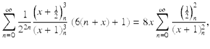
A few years ago Jésus Guillera found various Ramanujan-like identities for π, using integer relation methods. The three most basic—and entirely rational—identities are:

(8)

(9)

(10)

where .

Guillera proved (8) and (9) in tandem, by very ingeniously using the Wilf-Zeilberger algorithm [46, 52] for formally proving hypergeometric-like identities [24, 25, 35, 54]. No other proof is known, and there seem to be no like formulae for 1∕π ^N with N ≥ 4. The third, (10), is almost certainly true. Guillera ascribes (10) to Gourevich, who used integer relation methods to find it.

We were able to “discover” (10) using 30-digit arithmetic, and we checked it to 500 digits in 10 seconds, to 1200 digits in 6.25 minutes, and to 1500 digits in 25 minutes, all with naive command-line instructions in Maple. But it has no proof, nor does anyone have an inkling of how to prove it. It is not even clear that proof techniques used for (8) and (9) are relevant here, since, as experiment suggests, it has no “mate” in analogy to (8) and (9) [11]. Our intuition is that if a proof exists, it is more a verification than an explication, and so we stopped looking. We are happy just to “know” that the beautiful identity is true (although it would be more remarkable were it eventually to fail). It may be true for no good reason—it might just have no proof and be a very concrete Gödel-like statement.

There are other sporadic and unexplained examples based on other Pochhammer symbols, most impressively there is an unproven 2010 integer relation discovery by Cullen:

(11)

2.7 π without reciprocals

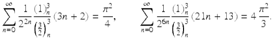
In 2008 Guillera [35] produced another lovely pair of third-millennium identities—discovered with integer relation methods and proved with creative telescoping—this time for π ² rather than its reciprocal. They are

(12)

and

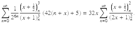
(13)

Here is the rising factorial. Substituting in (12) and (13), he obtained respectively the formulae

2.8 Quartic algorithm for π

One measure of the dramatic increase in computer power available to experimental mathematicians is the fact that the record for computation of π has gone from 29.37 million decimal digits in 1986 to 12.1 trillion digits in 2013. These computations have typically involved Ramanujan’s formula (6), the Chudnovsky formula (7), the Salamin-Brent algorithm [24, Ch. 3], or the Borwein quartic algorithm. The Borwein quartic algorithm, which was discovered by one of us and his brother Peter in 1983, with the help of a 16 Kbyte Radio Shack portable system, is the following: Set and , then iterate

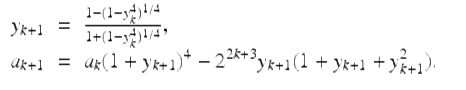
(14)

Then a _k converges quartically to 1∕π: each iteration approximately quadruples the number of correct digits. Twenty-two full-precision iterations of (14) produce an algebraic number that coincides with π to well more than 24 trillion places. Here is a highly abbreviated chronology of computations of π (based on http://en.wikipedia.org/wiki/Chronology_of_computation_of_pi).

·  1986: One of the present authors used (14) to compute 29.4 million digits of π. This required 28 hours on one CPU of the new Cray-2 at NASA Ames Research Center. Confirmation using the Salamin-Brent scheme took another 40 hours. This computation uncovered hardware and software errors on the Cray-2.

·  Jan. 2009: Takahashi used (14) to compute 1.649 trillion digits (nearly 60,000 times the 1986 computation), requiring 73.5 hours on 1024 cores (and 6.348 Tbyte memory) of a Appro Xtreme-X3 system. Confirmation via the Salamin-Brent scheme took 64.2 hours and 6.732 Tbyte of main memory.

·  Apr. 2009: Takahashi computed 2. 576 trillion digits.

·  Dec. 2009: Bellard computed nearly 2.7 trillion decimal digits (first in binary), using (7). This required 131 days on a single four-core workstation armed with large amounts of disk storage.

·  Aug. 2010: Kondo and Yee computed 5 trillion decimal digits using (7). This was first done in binary, then converted to decimal. The binary digits were confirmed by computing 32 hexadecimal digits of π ending with position 4,152,410,118,610, using BBP-type formulas for π due to Bellard and Plouffe (see Section 2.9). Additional details are given at http://www.numberworld.org/misc_runs/pi-5t/announce_en.html. These digits appear to be “very normal.”

·  Dec. 2013: Kondo and Yee extended their computation to 12.1 trillion digits.⁵

Daniel Shanks, who in 1961 computed π to over 100,000 digits, once told Phil Davis that a billion-digit computation would be “forever impossible.” But both Kanada and the Chudnovskys achieved that in 1989. Similarly, the intuitionists Brouwer and Heyting appealed to the “impossibility” of ever knowing whether and where the sequence 0123456789 appears in the decimal expansion of π, in defining a sequence (x _k ) _k ∈ N which is zero in each place except for a one in the n-th place where the sequence first starts to occur if at all.

This sequence converges to zero classically but was not then well-formed intuitionistically. Yet it was found in 1997 by Kanada, beginning at position 17387594880. Depending on ones ontological perspective, either nothing had changed, or the sequence had always converged but we were ignorant of such fact, or perhaps the sequence became convergent in 1997.

As late as 1989, Roger Penrose ventured, in the first edition of his book The Emperor’s New Mind, that we likely will never know if a string of ten consecutive sevens occurs in the decimal expansion of π. Yet this string was found in 1997 by Kanada, beginning at position 22869046249.

Figure 2 shows the progress of π calculations since 1970, superimposed with a line that charts the long-term trend of Moore’s Law. It is worth noting that whereas progress in computing π exceeded Moore’s Law in the 1990s, it has lagged a bit in the past decade.

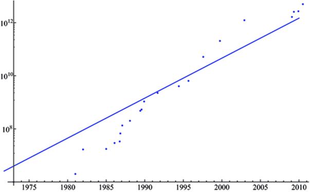
Fig. 2

Plot of π calculations, in digits (dots), compared with the long-term slope of Moore’s Law (line).

2.9 Digital integrity, II

There are many possible sources of errors in large computations of this type:

·  The underlying formulas and algorithms used might conceivably be in error, or have been incorrectly transcribed.

·  The computer programs implementing these algorithms, which necessarily employ sophisticated algorithms such as fast Fourier transforms to accelerate multiplication, may contain subtle bugs.

·  Inadequate numeric precision may have been employed, invalidating some key steps of the algorithm.

·  Erroneous programming constructs may have been employed to control parallel processing. Such errors are very hard to detect and rectify, since in many cases they cannot easily be replicated.

·  Hardware errors may have occurred in the middle of the run, rendering all subsequent computation invalid. This was a factor in the 1986 computation of π, as noted above.

·  Quantum-mechanical errors may have corrupted the results, for example, when a stray subatomic particle interacts with a storage register [50].

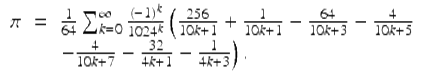
So why should anyone believe the results of such calculations? The answer is that such calculations are always double-checked with an independent calculation done using some other algorithm, sometimes in more than one way. For instance, Kanada’s 2002 computation of π to 1.3 trillion decimal digits involved first computing slightly over one trillion hexadecimal (base-16) digits, using (14). He found that the 20 hex digits of π beginning at position 10¹² + 1 are B4466E8D21 5388C4E014.

Kanada then calculated these same 20 hex digits directly, using the “BBP” algorithm [18]. The BBP algorithm for π is based on the formula

(15)

which was discovered via the PSLQ integer relation algorithm [24, pp. 232–234]. In particular, PSLQ discovered the formula

(16)

where is a Gaussian hypergeometric function. From (16), the series (15) almost immediately follows. The BBP algorithm, which is based on (15), permits one to calculate binary or hexadecimal digits of π beginning at an arbitrary starting point, without needing to calculate any of the preceding digits, by means of a simple scheme that requires only modest-precision arithmetic.

The result of the BBP calculation was B4466E8D21 5388C4E014. Needless to say, in spite of the many potential sources of error in both computations, the final results dramatically agree, thus confirming in a convincing albeit heuristic sense that both results are almost certainly correct. Although one cannot rigorously assign a “probability” to this event, note that the probability that two 20-long random hex digit strings perfectly agree is one in .

This raises the following question: Which is more securely established, the assertion that the hex digits of π in positions 10¹² + 1 through 10¹² + 20 are B4466E8D21 5388C4E014, or the final result of some very difficult work of mathematics that required hundreds or thousands of pages, that relied on many results quoted from other sources, and that (as is frequently the case) has been read in detail by only a relative handful of mathematicians besides the author? (See also [24, §8.4]). In our opinion, computation often trumps cerebration.

In a 2010 computation using the BBP formula, Tse-Wo Zse of Yahoo! Cloud Computing calculated 256 binary digits of π starting at the two quadrillionth bit. He then checked his result using the following variant of the BBP formula due to Bellard:

(17)

In this case, both computations verified that the 24 hex digits beginning immediately after the 500 trillionth hex digit (i.e., after the two quadrillionth binary bit) are: E6C1294A ED40403F 56D2D764.

In 2012 Ed Karrel using the BBP formula on the CUDA ⁶ system with processing to determine that starting after the 10¹⁵ position the hex-bits are E353CB3F7F0C9ACCFA9AA215F2. This was done on four NVIDIA GTX 690 graphics cards (GPUs) installed in CUDA. Yahoo!’s run took 23 days; this took 37 days.⁷

Some related BBP-type computations of digits of π ² and Catalan’s constant are described in [17]. In each case, the results were computed two different ways for validation. These runs used 737 hours on a 16384-CPU IBM Blue Gene computer, or, in other words, a total of 1378 CPU-years.

2.10 Formal verification of proof

In 1611, Kepler described the stacking of equal-sized spheres into the familiar arrangement we see for oranges in the grocery store. He asserted that this packing is the tightest possible. This assertion is now known as the Kepler conjecture, and has persisted for centuries without rigorous proof. Hilbert implicitly included the irregular case of the Kepler conjecture in problem 18 of his famous list of unsolved problems in 1900: whether there exist non-regular space-filling polyhedra? the regular case having been disposed of by Gauss in 1831.

In 1994, Thomas Hales, now at the University of Pittsburgh, proposed a five-step program that would result in a proof: (a) treat maps that only have triangular faces; (b) show that the face-centered cubic and hexagonal-close packings are local maxima in the strong sense that they have a higher score than any Delaunay star with the same graph; (c) treat maps that contain only triangular and quadrilateral faces (except the pentagonal prism); (d) treat maps that contain something other than a triangular or quadrilateral face; and (e) treat pentagonal prisms.

In 1998, Hales announced that the program was now complete, with Samuel Ferguson (son of mathematician-sculptor Helaman Ferguson) completing the crucial fifth step. This project involved extensive computation, using an interval arithmetic package, a graph generator, and Mathematica. The computer files containing the source code and computational results occupy more than three Gbytes of disk space. Additional details, including papers, are available at http://www.math.pitt.edu/~thales/kepler98. For a mixture of reasons—some more defensible than others—the Annals of Mathematics initially decided to publish Hales’ paper with a cautionary note, but this disclaimer was deleted before final publication.

Hales [36] has now embarked on a multi-year program to certify the proof by means of computer-based formal methods, a project he has named the “Flyspeck” project.⁸ As these techniques become better understood, we can envision a large number of mathematical results eventually being confirmed by computer, as instanced by other articles in the same issue of the Annals as Hales’ article. But this will take decades.

3 The experimental paradigm in applied mathematics

The field of applied mathematics is an enormous edifice, and we cannot possibly hope, in this short essay, to provide a comprehensive survey of current computational developments. So we shall limit our discussion to what may be termed “experimental applied mathematics,” namely employ methods akin to those mentioned above in pure mathematics to problems that had their origin in an applied setting. In particular, we will touch mainly on examples that employ either high-precision computation or integer relation detection, as these tools lead to issues similar to those already highlighted above.

First we will examine some historical examples of this paradigm in action.

3.1 Gravitational boosting or “slingshot magic”

One interesting space-age example is the unexpected discovery of gravitational boosting by Michael Minovitch, who at the time (1961) was a student working on a summer project at the Jet Propulsion Laboratory in Pasadena, California. Minovitch found that Hohmann transfer ellipses were not, as then believed, the minimum-energy way to reach the outer planets. Instead, he discovered, by a combination of clever analytical derivations and heavy-duty computational experiments on IBM 7090 computers (which were the world’s most powerful systems at the time), that spacecraft orbits which pass close by other planets could gain a “slingshot effect” substantial boost in speed, compensated by an extremely small change in the orbital velocity of the planet, on their way to a distant location [44]. Some of his earlier computation was not supported enthusiastically by NASA. As Minovitz later wrote,

Prior to the innovation of gravity-propelled trajectories, it was taken for granted that the rocket engine, operating on the well-known reaction principle of Newton’s Third Law of Motion, represented the basic, and for all practical purposes, the only means for propelling an interplanetary space vehicle through the Solar System.⁹

Without such a boost from Jupiter, Saturn, and Uranus, the Voyager mission would have taken more than 30 years to reach Neptune; instead, Voyager reached Neptune in only ten years. Indeed, without gravitational boosting, we would still be waiting! We would have to wait much longer for Voyager to leave the solar system as it now apparently is.

3.2 Fractals and chaos

One premier example of 20th century applied experimental mathematics is the development of fractal theory, as exemplified by the works of Benoit Mandelbrot. Mandelbrot studied many examples of fractal sets, many of them with direct connections to nature. Applications include analyses of the shapes of coastlines, mountains, biological structures, blood vessels, galaxies, even music, art, and the stock market. For example, Mandelbrot found that the coast of Australia, the West Coast of Britain, and the land frontier of Portugal all satisfy shapes given by a fractal dimension of approximately 1.75.

In the 1960s and early 1970s, applied mathematicians began to computationally explore features of chaotic iterations that had previously been studied by analytic methods. May, Lorenz, Mandelbrot, Feigenbaum [43], Ruelle, York, and others led the way in utilizing computers and graphics to explore this realm, as chronicled, for example, in Gleick’s book Chaos: Making a New Science [33]. By now fractals have found nigh countless uses. In our own research [12] we have been looking at expectations over self-similar fractals, motivated by modelling rodent brain-neuron geometry.

3.3 The uncertainty principle

Here we examine a principle that, while discovered early in the 20th century by conventional formal reasoning, could have been discovered much more easily with computational tools.

Most readers have heard of the uncertainty principle from quantum mechanics, which is often expressed as the fact that the position and momentum of a subatomic-scale particle cannot simultaneously be prescribed or measured to arbitrary accuracy. Others may be familiar with the uncertainty principle from signal-processing theory, which is often expressed as the fact that a signal cannot simultaneously be “time-limited” and “frequency-limited.” Remarkably, the precise mathematical formulations of these two principles are identical (although the quantum mechanics version presumes the existence of de Broglie waves).

Consider a real, continuously differentiable, L ² function f(t), which further satisfies as for some . (This assures convergence of the integrals below.) For convenience, we assume , so the Fourier transform of f(t) is real, although this is not necessary. Define

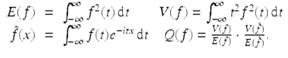
(18)

Then the uncertainty principle is the assertion that Q(f) ≥ 1∕4, with equality if and only if for real constants a and b. The proof of this fact is not terribly difficult but is hardly enlightening—see, for example, [24, pp. 183–188].

Let us approach this problem as an experimental mathematician might. As mentioned, it is natural when studying Fourier transforms (particularly in the context of signal processing) to consider the “dispersion” of a function and to compare this with the dispersion of its Fourier transform. Noting what appears to be an inverse relationship between these two quantities, we are led to consider Q(f) in (18). With the assistance of Maple or Mathematica, one can explore examples, as shown in Table 1. Note that each of the entries in the last column is in the range . Can one get any lower?

Table 1

Q values for various functions.

To further study this problem experimentally, note that the Fourier transform of f(t) can be closely approximated with a fast Fourier transform, after suitable discretization. The integrals V and E can be similarly evaluated numerically.

Then one can adopt a search strategy to minimize Q(f), starting, say, with a “tent function,” then perturbing it up or down by some ε on a regular grid with spacing , thus creating a continuous, piecewise linear function. When for a given δ, a minimizing function f(t) has been found, reduce ε and , and repeat. Terminate when δ is sufficiently small, say 10 ⁻⁶ or so. (For details, see [24].)

The resulting function f(t) is shown in Figure 3. Needless to say, its shape strongly suggests a Gaussian probability curve. Figure 3 actually shows both f(t) and the function , where b = 0. 45446177: they are identical to the resolution of the plot!

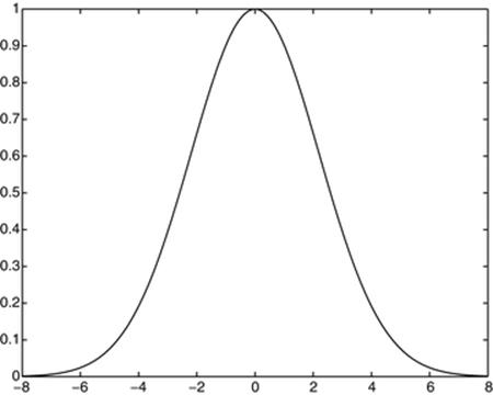
Fig. 3

Q-minimizer and matching Gaussian (identical to the plot resolution).

In short, it is a relatively simple matter, using 21st-century computational tools, to numerically “discover” the signal-processing form of the uncertainty principle. Doubtless the same is true of many other historical principles of physics, chemistry, and other fields, thus illustrating items 1, 2, 3, and 4 at the start of Section 2.

3.4 Chimera states in oscillator arrays

It is fair to say that the computational-experimental approach in applied mathematics has greatly accelerated in the 21st century. We show here a few specific illustrative examples. These include several by the present authors, because we are familiar with them. There are doubtless many others that we are not aware of that are similarly exemplary of the experimental paradigm.

One interesting example was the 2002 discovery by Kuramoto, Battogtokh, and Sima of “chimera” states, which arise in arrays of identical oscillators, where individual oscillators are correlated with oscillators some distance away in the array. These systems can arise in a wide range of physical systems, including Josephson junction arrays, oscillating chemical systems, epidemiological models, neural networks underlying snail shell patterns, and “ocular dominance stripes” observed in the visual cortex of cats and monkeys. In chimera states, named for the mythological beast that incongruously combines features of lions, goats, and serpents, the oscillator array bifurcates into two relatively stable groups, the first composed of coherent, phased-locked oscillators, and the second composed of incoherent, drifting oscillators.

According to Abrams and Strogatz, who subsequently studied these states in detail [1], most arrays of oscillators quickly converge into one of four typical patterns: (a) synchrony, with all oscillators moving in unison; (b) solitary waves in one dimension or spiral waves in two dimensions, with all oscillators locked in frequency; (c) incoherence, where phases of the oscillators vary quasi-periodically, with no global spatial structure; and (d) more complex patterns, such as spatiotemporal chaos and intermittency. But in chimera states, phase locking and incoherence are simultaneously present in the same system.

The simplest governing equation for a continuous one-dimensional chimera array is

(19)

where ϕ(x, t) specifies the phase of the oscillator given by x ∈ [0, 1) at time t, and G(x − x′) specifies the degree of nonlocal coupling between the oscillators x and x′. A discrete, computable version of (19) can be obtained by replacing the integral with a sum over a 1-D array (x _k , 0 ≤ k < N), where . Kuramoto and Battogtokh took for constant C and parameter κ.

Specifying , array size N = 256 and time step size , and starting from , where r is a uniform random variable on , gives rise to the phase patterns shown in Figure 4. Note that the oscillators near x = 0 and x = 1 appear to be phase-locked, moving in near-perfect synchrony with their neighbors, but those oscillators in the center drift wildly in phase, both with respect to their neighbors and to the locked oscillators.

Fig. 4

Phase of oscillations for a chimera system. The x-axis runs from 0 to 1 with periodic boundaries.

Numerous researchers have studied this phenomenon since its initial numerical discovery. Abrams and Strogatz studied the coupling function is given , where 0 ≤ A ≤ 1, for which they were able to solve the system analytically, and then extended their methods to more general systems. They found that chimera systems have a characteristic life cycle: a uniform phase-locked state, followed by a spatially uniform drift state, then a modulated drift state, then the birth of a chimera state, followed a period of stable chimera, then a saddle-node bifurcation, and finally an unstable chimera.¹⁰

3.5 Winfree oscillators

One closely related development is the resolution of the Quinn-Rand-Strogatz (QRS) constant. Quinn, Rand, and Strogatz had studied the Winfree model of coupled nonlinear oscillators, namely

(20)

for 1 ≤ i ≤ N, where is the phase of oscillator i at time t, the parameter κ is the coupling strength, and the frequencies ω _i are drawn from a symmetric unimodal density g(w). In their analyses, they were led to the formula

implicitly defining a phase offset angle due to bifurcation. The authors conjectured, on the basis of numerical evidence, the asymptotic behavior of the N-dependent solution s to be

where is now known as the QRS constant.

In 2008, the present authors together with Richard Crandall computed the numerical value of this constant to 42 decimal digits, obtaining

With this numerical value in hand, they were able to demonstrate that c ₁ is the unique zero of the Hurwitz zeta function on the interval . What’s more, they found that is given analytically by

In this case experimental computation led to a closed form which could then be used to establish the existence and form of the critical point, thus engaging at the very least each of items #1 through #6 of our ‘mathodology,’ and highlighting the interplay between computational discovery and theoretical understanding.

3.6 High-precision dynamics

Periodic orbits form the “skeleton” of a dynamical system and provide much useful information, but when the orbits are unstable, high-precision numerical integrators are often required to obtain numerically meaningful results.

For instance, Figure 5 shows computed symmetric periodic orbits for the (7 + 2)-Ring problem using double and quadruple precision. The (n + 2)-body Ring problem describes the motion of an infinitesimal particle attracted by the gravitational field of n + 1 primary bodies, n of them at the vertices of a regular n-gon rotating in its own plane about the central body with constant angular velocity. Each point corresponds to the initial conditions of one symmetric periodic orbit, and the grey area corresponds to regions of forbidden motion (delimited by the limit curve). To avoid “false” initial conditions it is useful to check if the initial conditions generate a periodic orbit up to a given tolerance level; but for highly unstable periodic orbits double precision is not enough, resulting in gaps in the figure that are not present in the more accurate quad precision run.

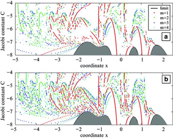
Fig. 5

Symmetric periodic orbits (m denotes multiplicity of the periodic orbit) in the most chaotic zone of the (7 + 2)-Ring problem using double (A) and quadruple (B) precision. Note “gaps” in the double precision plot. (Reproduced by permission.)

Hundred-digit precision arithmetic plays a fundamental role in a 2010 study of the fractal properties of the LORENZ ATTRACTOR [3.XY] (see Figure 6). The first plot shows the intersection of an arbitrary trajectory on the Lorenz attractor with the section z = 27, in a rectangle in the x − y plane. All later plots zoom in on a tiny region (too small to be seen by the unaided eye) at the center of the red rectangle of the preceding plot to show that what appears to be a line is in fact many lines.

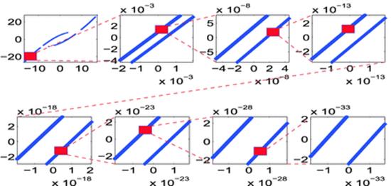
Fig. 6

Fractal property of the Lorenz attractor. (Reproduced by permission.)

The Lindstedt-Poincaré method for computing periodic orbits is based on the Lindstedt-Poincaré perturbation theory, Newton’s method for solving nonlinear systems, and Fourier interpolation. Viswanath has used this in combination with high-precision libraries to obtain periodic orbits for the Lorenz model at the classical Saltzman’s parameter values. This procedure permits one to compute, to high accuracy, highly unstable periodic orbits more efficiently than with conventional schemes, in spite of the additional cost of high-precision arithmetic. For these reasons, high-precision arithmetic plays a fundamental role in the study of the fractal properties of the Lorenz attractor (see Figures 6 and 7), and in the consistent formal development of complex singularities of the Lorenz system using infinite series. For additional details and references, see [5].

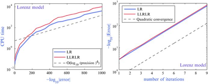
Fig. 7

Computational relative error vs. CPU time and number of iterations in a 1000-digit computation of the periodic orbits LR and LLRLR of the Lorenz model. (Reproduced by permission.)

3.7 Snow crystals

Computational experimentation has even been useful in the study of snowflakes. In a 2007 study, Janko Gravner and David Griffeath used a sophisticated computer-based simulator to study the process of formation of these structures, known in the literature as snow crystals and informally as snofakes. Their model simulated each of the key steps, including diffusion, freezing, and attachment, and thus enabled researchers to study, dependence on melting parameters. Snow crystals produced by their simulator vary from simple stars, to six-sided crystals with plate-ends, to crystals with dendritic ends, and look remarkably similar to natural snow crystals. Among the findings uncovered by their simulator is the fact that these crystals exhibit remarkable overall symmetry, even in the process of dynamically changing parameters. Their simulator is publicly available at http://psoup.math.wisc.edu/Snofakes.htm.

The latest developments in computer and video technology have provided a multiplicity of computational and symbolic tools that have rejuvenated mathematics and mathematics education. Two important examples of this revitalization are experimental mathematics and visual theorems. [38]

3.8 Visual mathematics

J. E. Littlewood (1885–1977) wrote [41]

A heavy warning used to be given [by lecturers] that pictures are not rigorous; this has never had its bluff called and has permanently frightened its victims into playing for safety. Some pictures, of course, are not rigorous, but I should say most are (and I use them whenever possible myself).

This was written in 1953, long before the current graphics, visualization and dynamic geometric tools (such as Cinderella or Geometer’s Sketchpad) were available.

The ability to “see” mathematics and mathematical algorithms as images, movies, or simulations is more-and-more widely used (as indeed we have illustrated in passing), but is still under appreciated. This is true for algorithm design and improvement and even more fundamentally as a tool to improve intuition, and as a resource when preparing or giving lectures (Fig. 8).

Fig. 8

Seeing often can and should be believing.

3.9 Iterative methods for protein conformation

In [2] we applied continuous convex optimization tools (alternating projection and alternating reflection algorithms) to a large class of non-convex and often highly combinatorial image or signal reconstruction problems. The underlying idea is to consider a feasibility problem that asks for a point in the intersection of two sets C ₁ and C ₂ in a Hilbert space.

The method of alternating projections (MAP) is to iterate

Here is the nearest point (metric) projection. The reflection is given by ), and the most studied Douglas-Rachford reflection method(DR) can be described by

This is nicely captured as ‘reflect-reflect-average.’

In practice, for any such method, one set will be convex and the other sequesters non-convex information.¹¹ It is most useful when projections on the two sets are relatively easy to estimate but the projection on the intersection Cis inaccessible. The methods often work unreasonably well but there is very little theory unless both sets are convex. For example, the optical aberration problem in the original Hubble telescope was ‘fixed’ by an alternating projection phase retrieval method (by Fienup and others), before astronauts could actually physically replace the mis-ground lens.

3.9.1 Protein conformation

We illustrate the situation with reconstruction of protein structure using only the short distances below about six Angstroms¹² between atoms that can be measured by nondestructive MRI techniques. This can viewed as a Euclidean distance matrix completion problem [2], so that only geometry (and no chemistry) is directly involved. That is, we ask the algorithm to predict a configuration in 3-space that is consistent with the given short distances.

What do the reconstructions look like? We turn to graphic information for 1PTQ and 1POA which were respectively our most and least successful cases.

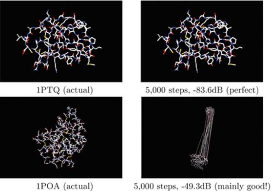
Note that the failure (and large mean or max error) is caused by a very few very large spurious distances¹³. The remainder is near perfect. Below we show the radical visual difference in the behavior of reflection and projection methods on IPTQ.

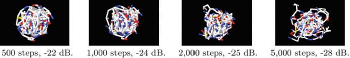
While traditional numerical measures (relative error in decibels, root mean square error, and maximum error) of success held some information, graphics-based tools have been dramatically more helpful. It is visually obvious that this method has successfully reconstructed the protein whereas the MAP reconstruction method, shown below, has not. This difference is not evident if one compares the two methods in terms of decibel measurement (beloved of engineers).

Douglas–Rachford reflection (DR) reconstruction: (of IPTQ¹⁴)

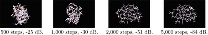
After 1000 steps or so, the protein shape is becoming apparent. After 2000 steps only minor detail is being fixed. Decibel measurement really does not discriminate this from the failure of the MAP method below which after 5000 steps has made less progress than DR after 1000.

Alternating projection (MAP) reconstruction: (of IPTQ)

Yet MAP works very well for optical abberation correction of the Hubble telescope and the method is now built in to amateur telescope software. This problem-specific variation in behavior is well observed but poorly understood; it is the heart of our current studies.

3.10 Mathematical finance

Coincident with the rise of powerful computational hardware, sophisticated mathematical techniques are now being employed to analyze market data in real-time and generate profitable investment strategies. This approach, commonly known as “quantitative” or “mathematical” finance, often involves computationally exploring a wide range of portfolio options or investment strategies [30, 40].

One interesting aspect of these studies is the increasing realization of how easy it is to “over-compute” an investment strategy, in a statistical sense. For example, one common approach to finding an effective quantitative investment strategy is to tune the strategy on historical data (a “backtest”). Unfortunately, financial mathematicians are finding that beyond a certain point, examining thousands or millions of variations of an investment strategy (which is certainly possible with today’s computer technology) to find the optimal strategy may backfire, because the resulting scheme may “overfit” the backtest data—the optimal strategy will work well only with a particular set of securities or over a particular time frame (in the past!). Indeed, backtest overfitting is now thought to be one of the primary reasons that an investment strategy which looks promising on paper often falls flat in real-world practice [15, 16].

3.11 Digital integrity III

Difficulties with statistical overfitting in financial mathematics can be seen as just one instance of the larger challenge of ensuring that results of computational experiments are truly valid and reproducible, which, after all, is the bedrock of all scientific research. We discussed these issues in the context of pure mathematics in Section 2.9, but there are numerous analogous concerns in applied mathematics:

·  Whether the calculation is numerically reproducible, i.e., whether or not the computation produces results acceptably close to those of an equivalent calculation performed using different hardware or software. In some cases, more stable numerical algorithms or higher-precision arithmetic may be required for certain portions of the computation to ameliorate such difficulties.

·  Whether the calculation has been adequately validated with independently written programs or distinct software tools.

·  Whether the calculation has been adequately validated by comparison with empirical data (where possible).

·  Whether the algorithms and computational techniques used in the calculation have been documented sufficiently well in journal articles or publicly accessible repositories, so that an independent researcher can reproduce the stated results.

·  Whether the code and/or software tool itself has been secured in a permanent repository.

These issues were addressed in a 2012 workshop held at the Institute for Computational and Experimental Research in Mathematics (ICERM). See [50] for details.

4 Additional examples of the experimental paradigm in action

4.1 Giuga’s conjecture

As another measure of what changes over time and what doesn’t, consider Giuga’s conjecture:

Giuga’s conjecture (1950): An integer n > 1, is a prime if and only if .

This conjecture is not yet proven. But it is known that any counterexamples are necessarily Carmichael numbers—square free ‘pseudo-prime numbers’—and much more. These rare birds were only proven infinite in number in 1994. In [25, pp. 227], we exploited the fact that if a number with m > 1 prime factors p _i is a counterexample to Giuga’s conjecture (that is, satisfies mod n), then for i ≠ j we have that p _i ≠ p _j , that

and that the p _i form a normal sequence: for i ≠ j. Thus, the presence of ‘3’ excludes and of ‘5’ excludes .

This theorem yielded enough structure, using some predictive experimentally discovered heuristics, to build an efficient algorithm to show—over several months in 1995—that any counterexample had at least 3459 prime factors and so exceeded 10¹³⁸⁸⁶, extended a few years later to 10¹⁴¹⁶⁴ in a five-day desktop computation. The heuristic is self-validating every time that the programme runs successfully. But this method necessarily fails after 8135 primes; at that time we hoped to someday exhaust its use.

In 2010, one of us was able to obtain almost as good a bound of 3050 primes in under 110 minutes on a laptop computer, and a bound of 3486 primes and 14,000 digits in less than 14 hours; this was extended to 3,678 primes and 17,168 digits in 93 CPU-hours on a Macintosh Pro, using Maple rather than C, which is often orders-of-magnitude faster but requires much more arduous coding. In 2013, the same one of us with his students revisited the computation and the time and space requirements for further progress [27]. Advances in multi-threading tools and good Python tool kits, along with Moore’s law, made the programming much easier and allowed the bound to be increased to 19,908 digits. This study also indicated that we are unlikely to exhaust the method in our lifetime.

4.2 Lehmer’s conjecture

An equally hard number-theory related conjecture, for which much less progress can be recorded, is the following. Here ϕ(n) is Euler’s totient function, namely the number of positive integers less than or equal to n that are relatively prime to n:

Lehmer’s conjecture (1932). if and only if n is prime. Lehmer called this “as hard as the existence of odd perfect numbers.”

Again, no proof is known of this conjecture, but it has been known for some time that the prime factors of any counterexample must form a normal sequence. Now there is little extra structure. In a 1997 Simon Fraser M.Sc. thesis, Erick Wong verified the conjecture for 14 primes, using normality and a mix of PARI, C and Maple to press the bounds of the “curse of exponentiality.” This very clever computation subsumed the entire scattered literature in one computation, but could only extend the prior bound from 13 primes to 14.

For Lehmer’s related 1932 question: when does ϕ(n)∣(n + 1)?, Wong showed there are eight solutions with no more than seven factors (six-factor solutions are due to Lehmer). Let

with denoting the Fermat primes. The solutions are

and the rogue pair 4919055 and 6992962672132095, but analyzing just eight factors seems out of sight. Thus, in 70 years the computer only allowed the exclusion bound to grow by one prime.

In 1932 Lehmer couldn’t factor 6992962672132097. If it had been prime, a ninth solution would exist: since ϕ(n)|(n + 1) with n + 2 prime implies that satisfies ϕ(N)|(N + 1). We say couldn’t because the number is divisible by 73; which Lehmer—a father of much factorization literature–could certainly have discovered had he anticipated a small factor. Today, discovering that

is nearly instantaneous, while fully resolving Lehmer’s original question remains as hard as ever.

4.3 Inverse computation and Apéry-like series

Three intriguing formulae for the Riemann zeta function are

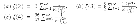
(21)

Binomial identity (21)(a) has been known for two centuries, while (b)—exploited by Apéry in his 1978 proof of the irrationality of ζ(3)—was discovered as early as 1890 by Markov, and (c) was noted by Comtet [11].

Using integer relation algorithms, bootstrapping, and the “Pade” function (Mathematica and Maple both produce rational approximations well), in 1996 David Bradley and one of us [11, 25] found the following unanticipated generating function for ζ(4n + 3):

(22)

Note that this formula permits one to read off an infinity of formulas for ζ(4n + 3), for beginning with (21)(b), by comparing coefficients of x ^4k on both sides of the identity.

A decade later, following a quite analogous but much more deliberate experimental procedure, as detailed in [11], we were able to discover a similar general formula for ζ(2n + 2) that is pleasingly parallel to (22):

(23)

As with (22), one can now read off an infinity of formulas, beginning with (21)(a). In 1996, the authors could reduce (22) to a finite form (24) that they could not prove,

(24)

but Almqvist and Granville did find a proof a year later. Both Maple and Mathematica can now prove identities like (24). Indeed, one of the values of such research is that it pushes the boundaries of what a CAS can do.

Shortly before his death, Paul Erdős was shown the form (24) at a meeting in Kalamazoo. He was ill and lethargic, but he immediately perked up, rushed off, and returned 20 minutes later saying excitedly that he had no idea how to prove (24), but that if proven it would have implications for the irrationality of ζ(3) and ζ(7). Somehow in 20 minutes an unwell Erdős had intuited backwards our whole discovery process. Sadly, no one has yet seen any way to learn about the irrationality of ζ(4n + 3) from the identity, and Erdős’s thought processes are presumably as dissimilar from computer-based inference engines as Kasparov’s are from those of the best chess programs.

A decade later, the Wilf-Zeilberger algorithm [46, 52]—for which the inventors were awarded the Steele Prize—directly (as implemented inMaple) certified (23) [24, 25]. In other words, (23) was both discovered and proven by computer. This is the experimental mathematician’s “holy grail” (item 6 in the list at the beginning of Section 2), though it would have been even nicer to be led subsequently to an elegant human proof. That preference may change as future generations begin to take it for granted that the computer is a collaborator [7].

We found a comparable generating function for , giving (21) (c) when x = 0, but one for still eludes us.

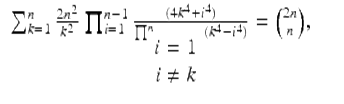
4.4 Ising integrals

High precision has proven essential in studies with Richard Crandall (see [9, 24]) of the following integrals:

where , and . Note that .

The D _n arise in the Ising theory of mathematical physics and the C _n in quantum field theory. As far as we know the E _n are an entirely mathematical construct introduced to study D _n . Direct computation of these integrals from their defining formulas is very difficult, but for C _n it can be shown that

where K ₀ is the modified Bessel function. Indeed, it is in this form that C _n arises in quantum field theory, as we subsequently learned from David Broadhurst. We had introduced it to study D _n . Again an uncanny parallel arises between mathematical inventions and physical discoveries.

Then 1000-digit numerical values so computed were used with PSLQ to deduce results such as , and furthermore to discover that

with additional higher-order terms in an asymptotic expansion. One intriguing experimental result (not then proven) is the following:

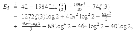
(25)

found by a multi-hour computation on a highly parallel computer system, and confirmed to 250-digit precision. Here is the standard order-4 polylogarithm. We also provided 250 digits of E ₆.

In 2013 Erik Panzer was able to formally evaluate all the E _n in terms of the alternating multi zeta values [45]. In particular, the experimental result for E ₅ was confirmed, and our high-precision computation of E ₆ was used to confirm Panzer’s evaluation

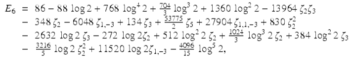
(26)

where ζ ₃ is a short hand for ζ(3) etc.

Here again we see true experimental applied mathematics, wherein our conjecture (25) and our numerical data for (26) (think of this as prepared biological sample) was used to confirm further discovery and proof by another researcher. Equation (26) was automatically converted to Latex from Panzer’s Maple worksheet.

Maple does a lovely job of producing correct but inelegant TE X. In our experience many (largely predictable) errors creep in while trying to prettify such output. For example, as in (1), while 704∕3 might have been 70∕43, it is less likely that a basis element is entirely garbled (although a power might be wrong). Errors are more likely to occur in trying to directly handle the TE X for complex expressions produced by computer algebra systems.

4.5 Ramble integrals and short walks

Consider, for complex s, the n-dimensional ramble integrals [10]

(27)

which occur in the theory of uniform random walk integrals in the plane, where at each step a unit-step is taken in a random direction as first studied by Pearson (who did discuss ‘rambles’), Rayleigh and others a hundred years ago. Integrals such as (27) are the s-th moment of the distance to the origin after n steps. As is well known, various types of random walks arise in fields as diverse as aviation, ecology, economics, psychology, computer science, physics, chemistry, and biology.

In 2010–2012 work (by J. Borwein, A. Straub, J. Wan and W. Zudilin), using a combination of analysis, probability, number theory and high-precision numerical computation, produced results such as

were obtained, where J _n (x) denotes the Bessel function of the first kind. These results, in turn, lead to various closed forms and have been used to confirm, to 600-digit precision, the following Mahler measure conjecture adapted from Villegas:

where the Dedekind eta-function can be computed from: η(q) = 

There are remarkable and poorly understood connections between diverse parts of pure, applied and computational mathematics lying behind these results. As often there is a fine interplay between developing better computational tools—especially for special functions and polylogarithms—and discovering new structure.

4.6 Densities of short walks

One of the deepest 2012 discoveries is the following closed form for the radial density of a four step uniform random walk in the plane: For 2 ≤ α ≤ 4 one has the real hypergeometric form:

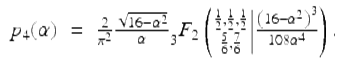
Remarkably, p ₄(α) is equal to the real part of the right side of this identity everywhere on [0, 4] (not just on [2, 4]), as plotted in Figure 9.

Fig. 9

The “shark-fin” density of a four step walk.

This was an entirely experimental discovery—involving at least one fortunate error—but is now fully proven.

4.7 Moments of elliptic integrals

The previous study on ramble integrals also led to a comprehensive analysis of moments of elliptic integral functions of the form:

where the elliptic functions K, E and their complementary versions are

Computations of these integrals to 3200-digit precision, combined with searches for relations using the PSLQ algorithm, yielded thousands of unexpected relations among these integrals (see [10]). The scale of the computation was required by the number of integrals under simultaneous investigation.

4.8 Computation and Constructivism

The fact that

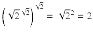
provides a one line proof that there exist irrational numbers α and β such that α ^β is rational. Indeed, either (a) is rational or (b) it is irrational; and can play the role of α. This lovely example of the principle of the excluded middle is rejected by constructivists and intuitionists alike. Indeed (b) holds but a constructive proof of such fact is quite elaborate. This is discussed in more detail in [24, §2.9] and [22].

Here we want to make the point that a computational sensibility leads one to want to know which case occurs, both for existential reasons, and because any algorithm with a conditional (if–then) step is probably worthless if one cannot determine which step to take.

4.9 Limits of computation

As we noted above, experimental studies have raised the question of whether one can truly trust—in the mathematical sense—the result of a computation, since there are many possible sources of errors: unreliable numerical algorithms; bug-ridden computer programs implementing these algorithms; system software or compiler errors; hardware errors, either in processing or storage; insufficient numerical precision; and obscure errors of hardware, software or programming that surface only in particularly large or difficult computations. Thus when applying experimental methods, it is essential to utilize rigorous validity checks, such as computing a key result by two completely different algorithms, and verifying that they produce the same result.

Along this line, it is important to keep in mind that even high-precision numerical evaluations can sometimes mislead. One remarkable example is the following:

(28)

The computation of this integral to high precision can be performed using a scheme described in [14]. When we first did this computation, we thought that the result was π∕8, but upon careful checking with the numerical value

it is clear that the two values disagree beginning with the 43rd digit!

The late Richard Crandall [29, §7.3] later explained this mystery. By employing a physically motivated analysis of running out of fuel random walks, he showed that π∕8 is given by the following very rapidly convergent series expansion, of which formula (28) above is merely the first term:

(29)

Two terms of the series above suffice for 500-digit agreement.

As a final sobering example in this section, we offer the following “sophomore’s dream” identity

(30)

where the denominators range over the odd primes, which was first discovered empirically. More generally, consider

(31)

Provably, the following is true: The “sum equals integral” identity, for remains valid at least for p among the first 10¹⁷⁶ primes; but stops holding after some larger prime, and thereafter the “sum less the integral” is strictly positive, but they always differ by much less than one part in a googol = 10 ¹⁰⁰. An even stronger estimate is possible assuming the Generalized Riemann Hypothesis (see [29, §7] and [19]).What does it mean for an identity to be provably false but, assuming that the universe is finite, at a level that is intrinsically infinitesimal?

As a single example of the sorts of difficulties that can arise even when one relies on well-maintained commercial software, the present authors found that neither Maple nor Mathematica was able to numerically evaluate constants of the form

where (for m, n, p, q ≥ 0 integers) to high precision in reasonable run time. In part this was because of the challenge of computing polylog and polylog derivatives (with respect to order) at complex arguments. The version of Mathematica that we were using was able to numerically compute to high precision, which is required here, but such evaluations were not only many times slower than Li _s (z) itself, but in some cases did not even return a tenth of the requested number of digits correctly [6].

For such reasons, experienced programmers of mathematical or scientific computations routinely insert validity checks in their code. Typically such checks take advantage of known high-level mathematical facts, such as the fact that the product of two matrices used in the calculation should always give the identity, or that the results of a convolution of integer data, done using a fast Fourier transform, should all be very close to integers.

5 Concluding Remarks

Let us start by reminding ourselves that in matters of practice what we do and what we say we do are not to be conflated. As Irving Kaplansky (1917–2006) remarked [37]:

We [Kaplansky and Halmos] share a philosophy about linear algebra: we think basis-free, we write basis-free, but when the chips are down we close the office door and compute with matrices like fury.

The central issues of how to view experimentally discovered results have been discussed before. In 1993, Arthur Jaffe and Frank Quinn warned of the proliferation of not-fully-rigorous mathematical results and proposed a framework for a “healthy and positive” role for “speculative” mathematics [39]. Numerous well-known mathematicians responded [3]. Morris Hirsch, for instance, countered that even Gauss published incomplete proofs, and the 15,000 combined pages of the proof of the classification of finite groups raises questions as to when we should certify a result. He suggested that we attach a label to each proof—e.g., “computer-aided,” “mass collaboration,” “constructive,” etc. Saunders Mac Lane quipped that “we are not saved by faith alone, but by faith and works,” meaning that we need both intuitive work and precision.

At the same time, computational tools now offer remarkable facilities to confirm analytically established results, as in the tools in development to check identities in equation-rich manuscripts, and in Hales’ project to establish the Kepler conjecture by formal methods.

The flood of information and tools in our information-soaked world is unlikely to abate. Thus in today’s computer-rich world it is essential to learn and teach judgment when it comes to using what is possible digitally. This means mastering the sorts of techniques we have illustrated and having some idea why a software system does what it does. It requires knowing when a computation is or can—in principle or practice—be made into a rigorous proof and when it is only compelling evidence (or is, in fact, entirely misleading). For instance, even the best commercial linear programming packages of the sort used by Hales will not certify any solution, although the codes are almost assuredly correct.

An effective digital approach to mathematics also requires rearranging hierarchies of what we view as hard and as easy. Continued fractions, moderate size integer or polynomial factorization, matrix decompositions, semi-definite programs, etc. are very different objects in vivo and in silico (see [24, Ch. 8, ed. 2]). It also requires developing a curriculum that carefully teaches experimental computer-assisted mathematics, either as a stand-alone course or as part of a related course in number theory or numerical methods. Some efforts along this line are already underway, mostly at the undergraduate level, by Marc Chamberland at Grinnell (http://www.math.grin.edu/~chamberl/courses/MAT444/syllabus.html), Victor Moll at Tulane, Jan de Gier in Melbourne, and Ole Warnaar at University of Queensland.

Judith Grabner has noted that a large impetus for the development of modern rigor in mathematics came with the Napoleonic introduction of regular courses: lectures and textbooks force a precision and a codification that apprenticeship obviates. But it will never be the case that quasi-inductive mathematics supplants proof. We need to find a new equilibrium. That said, we are only beginning to tap new ways to enrich mathematics. As Jacques Hadamard said more eloquently in French [47]:

The object of mathematical rigor is to sanction and legitimize the conquests of intuition, and there was never any other object for it.

Often in our experience, we follow a path empirically, computationally (numerically, graphically and symbolically) to a dead-end with a correct but unhelpful result. With non-traditional methods of rigor such as we have illustrated, in those cases we have frequently been spared proving intermediate results which while hard are ultimately sterile (i.e., item 5 in the list at the start of Section 2).

Never have we had such a cornucopia of ways to generate intuition. The challenge is to learn how to harness them, how to develop and how to transmit the necessary theory and practice. The Priority Research Centre for Computer Assisted Research Mathematics and its Applications (CARMA), http://www.newcastle.edu.au/research/centres/carmacentre.html, which one of us directs, hopes to play a lead role in this endeavor, an endeavor which in our view encompasses an exciting mix of exploratory experimentation and rigorous proof. And an exciting development showing the growing centrality of experimental mathematics is the opening of an NSF funded Institute for Computational and Experimental Research in Mathematics (ICERM), http://icerm.brown.edu/:

The mission of the Institute for Computational and Experimental Research in Mathematics (ICERM) is to support and broaden the relationship between mathematics and computation: specifically, to expand the use of computational and experimental methods in mathematics, to support theoretical advances related to computation, and address problems posed by the existence and use of the computer through mathematical tools, research and innovation.

Finally, it seems clear to us that experimental computation can end up reinforcing either an idealist or a constructivist approach, largely depending on one’s prior inclinations [42]. It is certainly both a supplement and a complement to traditional post-Cauchy modes of rigor. Experimental computation is also an interrogable lingua franca, allowing quite disparate parts of mathematics to more fruitfully entangle. For this we should all be very grateful.

References

1.

D. M. Abrams and S. H. Strogatz, “Chimera states in a ring of nonlocally coupled oscillators,” Intl. J. of Bifur. and Chaos, vol. 16 (2006), 21–37.MATHMathSciNetCrossRef

2.

F. Aragon, J. M. Borwein and M. Tam, “Douglas-Rachford feasibility methods for matrix completion problems.” ANZIAM Journal, July 2014, http://arxiv.org/abs/1308.4243.

3.

M. Atiyah, et al, “Responses to ‘Theoretical Mathematics: Toward a Cultural Synthesis of Mathematics and Theoretical Physics,’ by A. Jaffe and F. Quinn,” Bulletin of the American Mathematical Society, vol. 30, no. 2 (Apr 1994), 178–207.MATHMathSciNetCrossRef

4.

J. Avigad, “Computers in mathematical inquiry,” in The Philosophy of Mathematical Practice, P. Mancuso ed., Oxford University Press, 2008, 302–316.CrossRef

5.

D. H. Bailey, R. Barrio and J. M. Borwein, “High-precision computation: Mathematical physics and dynamics,” Appl. Math. and Comp., vol. 218 (2012), 10106–10121.MATHMathSciNetCrossRef

6.

D. H. Bailey and J. M. Borwein, “Computation and theory of extended Mordell-Tornheim-Witten sums. Part II,” Journal of Approximation Theory (special issue in honour of Dick Askey turning 80), vol. 189 (2015), 115–140. DOI: http://dx.doi.org/10.1016/j.jat.2014.10.004.

7.

D. H. Bailey and J. M. Borwein, “Computer-assisted discovery and proof.” Tapas in Experimental Mathematics, 21–52, in Contemporary Mathematics, vol. 457, American Mathematical Society, Providence, RI, 2008.

8.

D. H. Bailey and J. M. Borwein, “Experimental Applied Mathematics.” As a Final Perspective in the Princeton Companion to Applied Mathematics. Entry VIII.6, 925–932, 2015.

9.

D. H. Bailey and J. M. Borwein, “Exploratory experimentation and computation,” Notices of the AMS, vol. 58 (Nov 2011), 1410–19.MATHMathSciNet

10.

D. H. Bailey and J. M. Borwein, “Hand-to-hand combat with thousand-digit integrals,” J. Comp. Science, vol. 3 (2012), 77–86.CrossRef

11.

D. Bailey, J. Borwein, N. Calkin, R. Girgensohn, R. Luke and V. Moll, Experimental Mathematics in Action, A K Peters, Natick, MA, 2007.MATH

12.

D. Bailey, J. Borwein, R. Crandall and M. Rose, “Expectations on Fractal Sets.” Applied Mathematics and Computation. vol. 220 (Sept), 695–721. DOI: http://dx.doi.org/10.1016/j.amc.2013.06.078.

13.

D. H. Bailey, J. M. Borwein and A. D. Kaiser, “Automated simplification of large symbolic expressions,” Journal of Symbolic Computation, vol. 60 (Jan 2014), 120–136, http://www.sciencedirect.com/science/article/pii/S074771711300117X.

14.

D. H. Bailey, J. M. Borwein, V. Kapoor and E. Weisstein,“Ten Problems in Experimental Mathematics,” American Mathematical Monthly, vol. 113, no. 6 (Jun 2006), 481–409.MATHMathSciNetCrossRef

15.

D. H. Bailey, J. M. Borwein, M. Lopez de Prado and Q. J. Zhu, “Pseudo-mathematics and financial charlatanism: The effects of backtest over fitting on out-of-sample performance,” Notices of the American Mathematical Society, May 2014, http://ssrn.com/abstract=2308659.

16.

D. H. Bailey, J. M. Borwein, M. Lopez de Prado and Q. J. Zhu, “The probability of backtest overfitting,” Financial Mathematics, to appear, March 2015. http://ssrn.com/abstract=2326253.

17.

D. H. Bailey, J. M. Borwein, A. Mattingly and G. Wightwick, “The Computation of Previously Inaccessible Digits of π ² and Catalan’s Constant,” Notices of the American Mathematical Society, vol. 60 (2013), no. 7, 844–854.

18.

D. H. Bailey, P. B. Borwein and S. Plouffe, “On the Rapid Computation of Various Polylogarithmic Constants,” Mathematics of Computation, vol. 66, no. 218 (Apr 1997), 903–913.MATHMathSciNetCrossRef

19.

R. Baillie, D. Borwein, and J. Borwein, “Some sinc sums and integrals,” American Math. Monthly, vol. 115 (2008), no. 10, 888–901.

20.

J. M. Borwein, “The Experimental Mathematician: The Pleasure of Discovery and the Role of Proof,” International Journal of Computers for Mathematical Learning, 10 (2005), 75–108. CECM Preprint 02:178; 264, http://docserver.carma.newcastle.edu.au/264.

21.

J. M. Borwein, “Exploratory Experimentation: Digitally-assisted Discovery and Proof,” in ICMI Study 19: On Proof and Proving in Mathematics Education, G. Hanna and M. de Villiers, eds., New ICMI Study Series, 15, Springer-Verlag, 2012, http://www.carma.newcastle.edu.au/jon/icmi19-full.pdf.

22.

J. M. Borwein, “Implications of Experimental Mathematics for the Philosophy of Mathematics,” Ch. 2 (33–61) and cover image in Proof and Other Dilemmas: Mathematics and Philosophy, Bonnie Gold and Roger Simons, eds., MAA Spectrum Series, July 2008. D-drive Preprint 280, http://www.carma.newcastle.edu.au/jon/implications.pdf.

23.

J. M. Borwein, “The SIAM 100 Digits Challenge,” Extended review in the Mathematical Intelligencer, vol. 27 (2005), 40–48.

24.

J. M. Borwein and D. H. Bailey, Mathematics by Experiment: Plausible Reasoning in the 21st Century, A K Peters, second edition, 2008.

25.

J. M. Borwein, D. H. Bailey and R. Girgensohn, Experimentation in Mathematics: Computational Roads to Discovery, A K Peters, Natick, MA, 2004.

26.

J. M. Borwein, O-Y. Chan and R. E. Crandall, “Higher-dimensional box integrals,” Experimental Mathematics, vol. 19 (2010), 431–435.

27.

J. M. Borwein, C. Maitland and M. Skerritt, “Computation of an improved lower bound to Giuga’s primality conjecture,” Integers 13 (2013) #A67, http://www.westga.edu/~integers/cgi-bin/get.cgi.

28.

J. M. Borwein, I. J. Zucker and J. Boersma, “The evaluation of character Euler double sums,” Ramanujan Journal, vol. 15 (2008), 377–405.MATHMathSciNetCrossRef

29.

R. E. Crandall, “Theory of ROOF Walks,” 2007, http://www.perfscipress.com/papers/ROOF11_psipress.pdf.

30.

D. Easley, M. Lopez de Prado and M. O’Hara, High-Frequency Trading, Risk Books, London, 2013.

31.

L. R. Franklin, “Exploratory Experiments,” Philosophy of Science, vol. 72 (2005), 888–899.CrossRef

32.

M. Giaquinto, Visual Thinking in Mathematics. An Epistemological Study, Oxford University Press, New York, 2007.

33.

J. Gleick, Chaos: The Making of a New Science, Viking Penguin, New York, 1987.MATH

34.

J. Gravner and D. Griffeath, “Modeling snow crystal growth: A three-dimensional mesoscopic approach,” Phys. Rev. E, vol. 79 (2009), 011601.CrossRef

35.

J. Guillera, “Hypergeometric identities for 10 extended Ramanujan-type series,” Ramanujan Journal, vol. 15 (2008), 219–234.MATHMathSciNetCrossRef

36.

T. C. Hales, “Formal Proof,” Notices of the American Mathematical Society, vol. 55, no. 11 (Dec. 2008), 1370–1380.MATHMathSciNet

37.

Paul Halmos, Celebrating 50 Years of Mathematics, Springer, 1991.

38.

G. Hanna and M. de Villiers (Eds.), On Proof and Proving in Mathematics Education, the 19th ICMI Study, New ICMI Study Series, 15, Springer-Verlag, 2012.

39.

A. Jaffe and F. Quinn, “‘Theoretical Mathematics’: Toward a Cultural synthesis of Mathematics and Theoretical Physics,” Bulletin of the American Mathematical Society, vol. 29, no. 1 (Jul 1993), 1–13.MATHMathSciNetCrossRef

40.

Mark Joshi, The Concepts and Practice of Mathematical Finance, Cambridge University Press, 2008.MATH

41.

J. E. Littlewood, A Mathematician’s Miscellany, Methuen, London, 1953, reprinted by Cambridge University Press, 1986.

42.

M. Livio, Is God a Mathematician?, Simon and Schuster, New York, 2009.

43.

B. B. Mandelbrot, The Fractal Geometry of Nature, W. H. Freeman, New York, 1982.MATH

44.

M. Minovitch, “A method for determining interplanetary free-fall reconnaissance trajectories,” JPL Tech. Memo TM-312-130, (23 Aug 1961), 38–44.

45.

Erik Panzer, “Algorithms for the symbolic integration of hyperlogarithms with applications to Feynman integrals,” http://arxiv.org/abs/1403.3385.

46.

M. Petkovsek, H. S. Wilf, D. Zeilberger, A = B, A K Peters, Natick, MA, 1996.MATH

47.

G. Pólya, Mathematical discovery: On understanding, learning, and teaching problem solving, (Combined Edition), New York, John Wiley and Sons, New York, 1981.MATH

48.

R. Preston, “The Mountains of Pi,” New Yorker, 2 Mar 1992, http://www.newyorker.com/archive/content/articles/050411fr_archive01.

49.

H. K. Sørenson, “Exploratory experimentation in experimental mathematics: A glimpse at the PSLQ algorithm,” in B. Lowe, ed., Philosophy of Mathematics: Sociological Aspects and Mathematical Practice, Thomas Muller, London, 20–10, 341–360.

50.

V. Stodden, D. H. Bailey, J. M. Borwein, R. J. LeVeque, W. Rider and W. Stein, “Setting the default to reproducible: Reproducibility in computational and experimental mathematics,” manuscript, 2 Feb 2013, http://www.davidhbailey.com/dhbpapers/icerm-report.pdf.

51.

H. S. Wilf, “Mathematics: An experimental science,” The Princeton Companion to Mathematics, Princeton University Press, 2008.

52.

H. S. Wilf and D. Zeilberger, “Rational Functions Certify Combinatorial Identities,” Journal of the American Mathematical Society, vol. 3 (1990), 147–158.MATHMathSciNetCrossRef

53.

S. Wolfram, A New Kind of Science, Wolfram Media, Champaign, IL, 2002.MATH

54.

W. Zudilin, “Ramanujan-type formulae for 1∕π: A second wind,” 19 May 2008, http://arxiv.org/abs/0712.

Footnotes

1

We borrow heavily from two of our recent prior articles [9] (‘pure’) and [8] (‘applied’). They are reused with the permission of the American Mathematical Society and of Princeton University Press, respectively.

2

Most of the functionality of the ISC, which is now housed at http://carma-lx1.newcastle.edu.au:8087, is now built into the “identify” function of Maple starting with version 9.5. For example, the Maple command identify(4.45033263602792) returns , meaning that the decimal value given is simply approximated by .

3

The difficulty of comparing timings and the growing inability to look under the hood (bonnet) in computer packages, either by design or through user ignorance, means all such comparisons should be taken with a grain of salt.

4

See http://fredrikj.net/blog/2014/03/new-partition-function-record/ for a lovely description of the computation of p(10²⁰), which has over 11 billion digits and required knowing π to similar accuracy.

5

See “12.1 Trillion Digits of Pi And we’re out of disk space…” at http://www.numberworld.org/misc_runs/pi-12t/.

6

See http://en.wikipedia.org/wiki/CUDA.

7

See www.karrels.org/pi/.

8

He reported in December 2012 at an ICERM workshop that this was nearing completion.

9

There are differing accounts of how this principle was discovered; we rely on the first-person account at http://www.gravityassist.com/IAF1/IAF1.pdf. Additional information on “slingshot magic” is given at http://www.gravityassist.com/ and http://www2.jpl.nasa.gov/basics/grav/primer.php.

10

Various movies can be found on line. For example, http://dmabrams.esam.northwestern.edu/pubs/ngeo-video1.mov and http://dmabrams.esam.northwestern.edu/pubs/ngeo-video2.mov show two for groundwater flow.

11

When the set A is non-convex the projection P _A (x) may be a set and we must instead select some .

12

Interatomic distances below 6Å typically constitute less than 8% of the total distances between atoms in a protein.

13

After speeding up the computation by a factor of ten, and terminating when the decibel error was less than − 100, this anomaly disappeared.

14

The first 3,000 steps of the 1PTQ reconstruction are available as a movie at http://carma.newcastle.edu.au/DRmethods/1PTQ.html.