Pre-Calculus For Dummies, 2nd Edition (2012)

Part III. Analytic Geometry and System Solving

Chapter 13. Streamlining Systems, Managing Variables

In This Chapter

Taking down two-equation systems with substitution and elimination

Breaking down systems with more than two equations

Graphing systems of inequalities

Forming and operating on matrices

When you have one variable and one equation, you can almost always solve the equation. Finding a solution may take you some time, but it is usually possible. When a problem has two variables, however, you need at least two equations to solve; this set of equations is called a system. When you have three variables, you need at least three equations in the system. Basically, for every variable present, you need a separate unique equation if you want to solve for it.

For an equation with three variables, an infinite number of values for two variables would work for that particular equation. Why? Because you can pick any two numbers to plug in for two of the variables in order to find the value of the third one that makes the equation true. If you add another equation into the mix, the solutions to the first equation now have to also work in the second equation, which makes for fewer solutions that work. The set of solutions (usually x, y, z, and so on) must work when plugged into each and every equation in the system. More equations mean fewer values work as solutions.

Of course, the bigger a system of equations becomes, the longer it takes to solve it algebraically. Therefore, certain systems are easier to solve in certain ways, which is why math books usually show several methods. In this chapter, we follow suit, showing you when each method is preferable to all the others. You want to be comfortable with as many of these methods as possible so that you can choose the best route possible, which is the one with the least number of steps (which means fewer places to get mixed up).

As if systems of equations weren’t enough on their own, in this chapter we also introduce you to systems of inequalities. These systems of inequalities require you to graph the solution, but you don’t need to find the exact values of the solutions — because they don’t exist. The solution to a system of inequalities is shown as a shaded region on a graph.

A Primer on Your System-Solving Options

Before you can know which method of solving is best, you need to be familiar with the possibilities. Your system-solving options are as follows:

If the system has only two or three variables, you can use substitution or elimination (which you have seen before in Algebra I and Algebra II).

If the system has four or more variables, you can use matrices, which are rectangular tables that display either numbers or variables, called elements. With matrices, you have your choice of the following approaches, all of which we discuss later in this chapter:

• Gaussian elimination

• Inverse matrices

• Cramer’s rule

A note to the calculator-savvy students out there: Some instructors teach the material contained in this chapter and tell students to just plug the numbers into a calculator, don’t ask any questions, and move on. If you’re lucky enough to have a graphing calculator and a calculator-happy teacher, you could let the calculator do the math for you. However, because we’re mathematicians, we always recommend that you buckle down and learn it anyway; then pat yourself on the back for going the extra mile!

No matter which system-solving method you use, check the answers you get, because even the best mathematicians make mistakes sometimes, and we learn a lot from our mistakes. The more variables and equations you have in a system, the more likely you are to make a mistake. And if you make a mistake in calculations somewhere, it can affect more than one answer, because one variable usually is dependent on another. Always verify!

Finding Solutions of Two-Equation Systems Algebraically

When you solve systems with two variables and therefore two equations, the equations can be linear or nonlinear. Linear systems are usually expressed in the form Ax + By = C, where A, B, and C are real numbers.

Nonlinear equations can include circles, other conics, polynomials, and exponential, logarithmic, or rational functions. Elimination won’t work in nonlinear systems if x appears in one equation of the system but x² appears in another equation, because the terms aren’t alike and therefore can’t be added together. In that case, you’re stuck with substitution to solve the nonlinear system.

Like most algebra problems, systems can have a number of possible solutions. If a system has one or more unique solutions that can be expressed as coordinate pairs, it’s called consistent and independent. If it has no solution, it’s called an inconsistent system. If the solutions are infinite, the system is called dependent. It can be difficult to tell which of these categories your system of equations falls into just by looking at the problem. A linear system can only have no solution, one solution, or infinite solutions, because two different straight lines can intersect in only one place (if you don’t believe us, draw a picture). A line and a conic section can intersect no more than twice, and two conic sections can intersect a maximum of four times.

Solving linear systems

When solving linear systems, you have two methods at your disposal, and which one you choose depends on the problem:

If the coefficient of any variable is 1, which means you can easily solve for it in terms of the other variable, then substitution is a very good bet. If you use this method, you can set up each equation any way you want.

If all the coefficients are anything other than 1, then you can use elimination, but only if the equations can be added together to make one of the variables disappear. However, if you use this method, be sure that all the variables and the equal sign line up with one another before you add the equations together.

With the substitution method

In the substitution method, you use one equation to solve for one variable and then substitute that expression into the other equation to solve for the other variable. To begin the easiest way, look for a variable with a coefficient of 1 to solve for. You just have to add or subtract terms in order to move everything to the other side of the equal sign, just like you’ve been doing to solve for variables since Algebra I. That way, you won’t have to divide by the coefficient when you’re solving, which means you won’t have any fractions.

For example, suppose you’re managing a theater and you need to know how many adults and children are in attendance at a show. The auditorium is sold out and contains a mixture of adults and children. The tickets cost $23.00 per adult and $15.00 per child. If the auditorium has 250 seats and the total ticket revenue for the event is $4,846.00, how many adults and children are in attendance?

To solve the problem with the substitution method, follow these steps:

1. Express the word problem as a system of equations.

You can use the information given in the word problem to set up two different equations. You want to solve for how many adult tickets (a) and child tickets (c) you sold. If the auditorium has 250 seats and was sold out, the sum of the adult tickets and child tickets must be 250.

The ticket prices also lead you to the revenue (or money made) from the event. The adult ticket price times the number of adults present lets you know how much money you made from the adults. You can do the same calculation with the child tickets. The sum of these two calculations must be the total ticket revenue for the event.

Here’s how you write this system of equations:

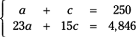
2. Solve for one of the variables.

Pick the variable with a coefficient of 1 if you can, because solving for this variable will be easy. For this example, you can choose to solve for a in the first equation. To do so, subtract c from both sides: a = 250 – c.

You can always move things from one side of an equation to the other, but don’t fall prey to the trap that 250 – c is 249c. Those terms are not like, so you can’t combine them.

3. Substitute the solved variable into the other equation.

In this example, you solve for a in the first equation. You take this value (250 – c) and substitute it into the other equation for a. (Make sure that you don’t substitute into the equation you used in Step 1; otherwise, you’ll be going in circles.)

The second equation now says 23(250 – c) + 15c = 4,846.

4. Solve for the unknown variable.

You distribute the number 23:

5,750 – 23c + 15c = 4,846

And then you simplify:

5,750 – 8c = 4,846, or –8c = –904

So c = 113. A total of 113 children attended the event.

5. Substitute the value of the unknown variable into one of the original equations to solve for the other unknown variable.

You don’t have to substitute into one of the original equations, but your answer is more likely to be accurate if you do.

When you plug 113 into the first equation for c, you get a + 113 = 250. Solving this equation, you get a = 137. You sold a total of 137 adult tickets.

6. Check your solution.

When you plug a and c into the original equations, you should get two true statements. Does 137 + 113 = 250? Yes. Does 23(137) + 15(113) = 4,846? Indeed.

By using the process of elimination

If solving a system of two equations with the substitution method proves difficult or the system involves fractions, the elimination method is your next best option. (Who wants to deal with fractions anyway?) In the elimination method, you make one of the variables cancel itself out by adding the two equations.

Sometimes you have to multiply one or both equations by constants in order to add the equations; this situation occurs when you can’t eliminate one of the variables by just adding the two equations together. (Remember that in order for one variable to be eliminated, the coefficients of one variable must be opposites.)

For example, the following steps show you how to solve this system by using the process of elimination:

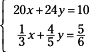
1. Rewrite the equations, if necessary, to make like variables line up underneath each other.

The order of the variables doesn’t matter; just make sure that like terms line up with like terms from top to bottom. The equations in this system have the variables x and y lined up already:

2. Multiply the equations by constants to make one set of variables match coefficients.

Decide which variable you want to eliminate.

Say you decide to eliminate the x-variables; first, you have to find their least common multiple. What number do 20 and 1/3 both go into? The answer is 60. But one of them has to be negative so that when you add the equations, the terms cancel out (that’s why it’s called elimination!). Multiply the top equation by –3 and the bottom equation by 180. (Be sure to distribute this number to each term — even on the other side of the equal sign.) Doing this step gives you the following equations:

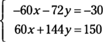
3. Add the two equations.

You now have 72y = 120.

4. Solve for the unknown variable that remains.

Dividing by 72 gives you y = 5/3.

5. Substitute the value of the found variable into either equation.

We chose the first equation: 20x + 24(5/3) = 10.

6. Solve for the final unknown variable.

You end up with x = –3/2.

7. Check your solutions.

Always verify your answer by plugging the solutions back into the original system. These check out!

20(–3/2) + 24(5/3) = –30 + 40 = 10

It works! Now check the other equation:

Because both values are solutions to both equations, the solution to the system is correct.

Working nonlinear systems

In a nonlinear system, at least one equation has a graph that isn’t a straight line. You can always write a linear equation in the form Ax + By = C (where A, B, and C are real numbers); a nonlinear system is represented by any other form. Examples of nonlinear equations include, but are not limited to, any conic section, polynomial, rational function, exponential, or logarithm (all of which we cover in other parts of this book). The nonlinear systems you’ll see in pre-calc have two equations with two variables, because the three-dimensional systems are extremely difficult to solve (trust us on that one!). Because you’re really working with a system with two equations and two variables (even though one or both equations are nonlinear), you have the same two methods at your disposal: substitution and elimination.

The method of solving nonlinear systems is different from that of linear systems in that these systems are much more complicated and therefore require much more work. (Those exponents really screw things up.) Unlike before (with linear systems), nonlinear systems are less forgiving than the systems we cover earlier in the chapter. Usually, substitution is your best bet. Unless the variable you want to eliminate is raised to the same power in both equations, elimination won’t get you anywhere.

When one system equation is nonlinear

If one equation in a system is nonlinear, your first thought before solving should be, “Bingo! Substitution method!” (or something to that effect). In this situation, you can solve for one variable in the linear equation and substitute this expression into the nonlinear equation, because solving for a variable in a linear equation is a piece of cake! And any time you can solve for one variable easily, you can substitute that expression into the other equation to solve for the other one.

For example, follow these steps to solve this system:

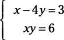
1. Solve the linear equation for one variable.

In the example system, the top equation is linear. If you solve for x, you get x = 3 + 4y.

2. Substitute the value of the variable into the nonlinear equation.

When you plug 3 + 4y into the second equation for x, you get (3 + 4y)y = 6.

3. Solve the nonlinear equation for the variable.

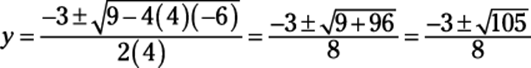
When you distribute the y, you get 4y² + 3y = 6. Because this equation is quadratic (refer to Chapter 4), you must get 0 on one side, so subtract the 6 from both sides to get 4y² + 3y – 6 = 0. You have to use the quadratic formula to solve this equation for y:

When you square root something, you get a positive and a negative answer, which means you have two different answers in this situation.

4. Substitute the solution(s) into either equation to solve for the other variable.

Because you find two solutions for y, you have to substitute them both to get two different coordinate pairs. Here’s what happens when you do:

If , then

If , then

Therefore, you get the solutions to the system:

and

These solutions represent the intersection of the line x – 4y = 3 and the rational function xy = 6.

When both system equations are nonlinear

If both of the equations in a system are nonlinear, well, you just have to get more creative to find the solutions. Unless one variable is raised to the same power in both equations, elimination is out of the question. Solving for one of the variables in either equation isn’t necessarily easy, but it can usually be done. After you solve for a variable, plug this expression into the other equation and solve for the other variable just as you did before. Unlike linear systems, many operations may be involved in the simplification or solving of these equations. Just remember to keep your order of operations in mind at each step of the way.

When both equations in a system are conic sections, you’ll never find more than four solutions (unless the two equations describe the same conic section, in which case the system has an infinite number of solutions — and therefore is a dependent system). Four is the limit because conic sections are all very smooth curves with no sharp corners or crazy bends, so two different conic sections can’t intersect more than four times.

For example, suppose a problem asks you to solve the following system:

Doesn’t that problem just make your skin crawl? Don’t break out the calamine lotion just yet, though. Follow these steps to find the solutions:

1. Solve for x² or y² in one of the given equations.

The second equation is attractive because all you have to do is add 9 to both sides to get y + 9 = x².

2. Substitute the value from Step 1 into the other equation.

You now have y + 9 + y² = 9. Aha! You have a quadratic equation, and you know how to solve that (from Chapter 4).

3. Solve the quadratic equation.

Subtract 9 from both sides to get y + y² = 0.

Remember that you’re not allowed, ever, to divide by a variable.

You must factor out the greatest common factor (GCF) instead to get y(1 + y) = 0. Use the zero product property to solve for y = 0 and y = –1. (Chapter 4 covers the basics of how to complete these tasks.)

4. Substitute the value(s) from Step 3 into either equation to solve for the other variable.

We chose to use the equation solved for in Step 1. When y is 0, 9 = x², so x = ±3. When y is –1, 8 = x², so .

Be sure to keep track of which solution goes with which variable, because you have to express these solutions as points on a coordinate pair. Your answers are (–3, 0), (3, 0), , and .

This solution set represents the intersections of the circle and the parabola given by the equations in the system.

Solving Systems with More than Two Equations

Larger systems of linear equations involve more than two equations that go along with more than two variables. These larger systems can be written in the form Ax + By + Cz + . . . = K where all coefficients (and K) are constants. These linear systems can have many variables, and you can solve those systems as long as you have one unique equation per variable. In other words, three variables need three equations to find a unique solution, four variables need four equations, and ten variables would have to have ten equations, and so on. You don’t need to concern yourself with larger systems of nonlinear equations. Those systems are far too complicated for pre-calc. For these types of nonlinear systems, the solutions you can find vary widely:

You may find no solution.

You may find one unique solution.

You may come across infinitely many solutions.

The number of solutions you find depends on how the equations interact with one another. Because linear systems of three variables describe equations of planes, not lines (as two-variable equations do), the solution to the system depends on how the planes lie in three-dimensional space relative to one another. Unfortunately, just like in the systems of equations with two variables, you can’t tell how many solutions the system has without doing the problem. Treat each problem as if it has one solution, and if it doesn’t, you will either arrive at a statement that is never true (no solutions) or is always true (which means the system has infinite solutions).

Typically, you must use the elimination method more than once to solve systems with more than two variables and two equations (see the earlier section “By using the process of elimination”).

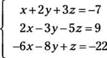
For example, suppose a problem asks you to solve the following system:

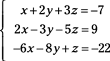
To find the solution(s), follow these steps:

1. Look at the coefficients of all the variables and decide which variable is easiest to eliminate.

With elimination, you want to find the least common multiple (LCM) for one of the variables, so go with the one that’s the easiest. In this case, we recommend that you eliminate the x-variable.

2. Set apart two of the equations and eliminate one variable.

Looking at the first two equations, you have to multiply the top by –2 and add it to the second equation. Doing this, you get the following equation:

3. Set apart another two equations and eliminate the same variable.

The first and the third equations allow you to easily eliminate x again. Multiply the top equation by 6 and add it to the third equation to get the following equation:

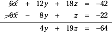
4. Repeat the elimination process with your two new equations.

You now have these two equations with two variables:

You need to eliminate one of these variables. We’ve chosen to eliminate the y-variable by multiplying the top equation by 4 and the bottom by 7 and then adding the equations. Here’s what that step gives you:

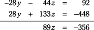
5. Solve the final equation for the variable that remains.

If 89z = –356, then z = –4.

6. Substitute the value of the solved variable into one of the equations that has two variables to solve for another one.

We chose the equation –7y – 11z = 23. Substituting, you have –7y – 11(–4) = 23, which simplifies to –7y + 44 = 23. Now finish the job:–7y = –21, y = 3.

7. Substitute the two values you now have into one of the original equations to solve for the last variable.

We chose the first equation in the original system, which now becomes x + 2(3) + 3(–4) = –7. Simplify to get your final answer:

x + 6 – 12 = –7

x – 6 = –7

x = –1

The solutions to this equation are x = –1, y = 3, and z = –4.

This process is called back substitution because you literally solve for one variable and then work your way backward to solve for the others (you see this process again later when solving matrices). In this last example, we went from the solution for one variable in one equation to two variables in two equations to the last step with three variables in three equations. Always move from the simpler to the more complicated.

Decomposing Partial Fractions

A process called partial fractions takes one fraction and expresses it as the sum or difference of two other fractions. We can think of many reasons why you’d need to do this. In calculus, this process is useful before you integrate a function. Because integration is so much easier when the degree of a rational function is 1 in the denominator, partial fraction decomposition is a useful tool for you.

The process of decomposing partial fractions requires you to separate the fraction into two (or sometimes more) disjointed fractions with variables (usually A, B, C, and so on) standing in as placeholders in the numerator. Then you can set up a system of equations to solve for these variables. For instance, you must follow these steps to write the partial fraction decomposition of the following fraction:

1. Factor the denominator (see Chapter 4) and rewrite it as A over one factor and B over the other.

You do this because you want to break the fraction into two. The process unfolds as follows:

2. Multiply every term you’ve created by the factored denominator and then cancel.

You’ll multiply a total of three times in this example:

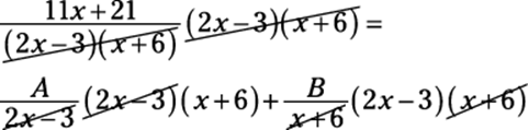
This expression equals the following:

11x + 21 = A(x + 6) + B(2x – 3)

3. Distribute A and B.

This step gives you

11x + 21 = Ax + 6A + 2Bx – 3B

4. On the right side of the equation only, put all terms with an x together and all terms without it together.

Rearranging gives you

11x + 21 = Ax + 2Bx + 6A – 3B

5. Factor out the x from the terms on the right side.

You now have

11x + 21 = (A + 2B)x + 6A – 3B

6. Create a system out of this equation by pairing up terms.

For an equation to work, everything must be in balance. Because of this fact, the coefficients of x must be equal and the constants must be equal. If the coefficient of x is 11 on the left and A + 2B on the right, you can say that 11 = A + 2B is one equation. Constants are the terms with no variable, and in this case, the constant on the left is 21. On the right side, 6A – 3B is the constant (because no variable is attached) and so 21 = 6A – 3B.

7. Solve the system, using either substitution or elimination (see the earlier sections of this chapter).

We use elimination in this system. You have the following equations:

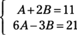
So you can multiply the top equation by –6 and then add to eliminate and solve. You find that A = 5 and B = 3.

8. Write the solution as the sum of two fractions.

Surveying Systems of Inequalities

In a system of inequalities, you see more than one inequality with more than one variable. Before pre-calculus, teachers tend to focus mostly on systems of linear inequalities. The graphs of those inequalities are straight lines. In pre-calc, though, you expand your study to systems of nonlinear inequalities because they are more thorough in the types of equations they cover (straight lines are so boring!).

In these systems of inequalities, at least one inequality isn’t linear. The only way to solve a system of inequalities is to graph the solution. Fortunately, these graphs look very similar to the graphs you have been graphing throughout your entire pre-calc course, and earlier. You may be required to graph inequalities that you haven’t seen since pre-algebra. But for the most part, these inequalities probably resemble the parent functions from Chapter 3 and conic sections from Chapter 12. The only difference between then and now is that the line that you graph is either solid or dashed, depending on the problem, and you get to color (or shade) where the solutions lie!

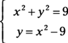
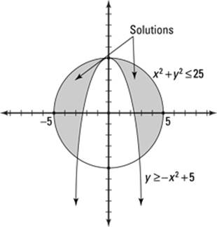
For example, consider the following nonlinear system of inequalities:

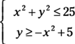
To solve this system of equations, first graph the system. The fact that these expressions are inequalities and not equations doesn’t change the general shape of the graph at all. Therefore, you can graph these inequalities just as you would graph them if they were equations. The top equation of this example is a circle (for a quick refresher on graphing circles, refer to Chapter 12 about conic sections). This circle is centered at the origin, and the radius is 5. The second equation is an upside-down parabola (there’s those pesky conic sections again!). It is shifted vertically 5 units and flipped upside down. Because both of the inequality signs in this example include the equality line underneath (the first one is “less than or equal to” and the second is “greater than or equal to”), both lines should be solid.

If the inequality symbol says “strictly greater than: >” or “strictly less than: <” then the boundary line for the curve (or line) should be dashed.

After graphing, pick one test point that isn’t on a boundary and plug it into the equations to see if you get true or false statements. The point that you pick as a solution must work in every equation.

For example, our test point is (0, 4). If you plug this point into the inequality for the circle (see Chapter 12), you get 0² + 4² ≤ 25. This statement is true because 16 ≤ 25, so you shade inside the circle. Now plug the same point into the parabola to get 4 ≥ –0² + 5, but because 4 isn’t greater than 5, this statement is false. You shade outside the parabola.

The solution of this system of inequalities is where the shading overlaps.

See Figure 13-1 for the final graph.

Introducing Matrices: The Basics

In the previous sections of this chapter, we cover how to solve systems of two or more equations by using substitution or elimination. But these methods get very messy when the size of a system rises above three equations. Not to worry; whenever you have four or more equations to solve simultaneously, matrices are your best bet.

A matrix is a rectangle of numbers arranged in rows and columns. You use matrices to organize complicated data — say, for example, you want to keep track of sales records in your store. Matrices help you do that, because they can separate the sales by day in columns while different types of sales are organized by row.

After you get comfortable with what matrices are and how they’re important, you can start adding, subtracting, and multiplying them by scalars and each other. Operating on matrices is useful when you need to add, subtract, or multiply large groups of data in an organized fashion. (Note: Matrix division doesn’t exist, so don’t spend time worrying about it.) This section shows you how to perform all the above operations.

One thing to always remember when working with matrices is the order of operations, which is the same across all math applications: First do any multiplication and then do the addition/subtraction.

You express the dimensions, sometimes called order, of a matrix as the number of rows by the number of columns. For example, if matrix M is 3 x 2, it has three rows and two columns.

To remember that rows come first, think of how you read in English — from left to right and then down, so the horizontal comes first.

Applying basic operations to matrices

Operating on matrices works very much like operating on multiple terms within parentheses; you just have more terms in the “parentheses” to work with. Just like with operations on numbers, a certain order is involved with operating on matrices. Multiplication comes before addition and/or subtraction. When multiplying by a scalar, a constant that multiplies a quantity (which changes its size, or scale), each and every element of the matrix gets multiplied. The following sections show you how to compute some of the more basic operations on matrices: addition, subtraction, and multiplication.

When adding or subtracting matrices, you just add or subtract their corresponding terms. It’s as simple as that. Figure 13-2 shows how to add and subtract two matrices.

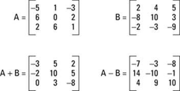
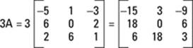
Note, however, that you can add or subtract matrices only if their dimensions are exactly the same. To add or subtract matrices, you add or subtract their corresponding terms; if the dimensions aren’t exactly the same, then the terms won’t line up. And obviously, you can’t add or subtract terms that aren’t there! When you multiply a matrix by a scalar, you’re just multiplying by a constant. To do that, you multiply each term inside the matrix by the constant on the outside. Using the same matrix A from the previous example, you can find 3A by multiplying each term of matrix A by 3. Figure 13-3 shows this example:

Suppose a problem asks you to combine operations. You simply multiply each matrix by the scalar separately and then add or subtract them. For example, consider the following two matrices:

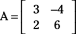
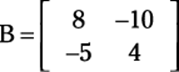
Find 3A – 2B as follows:

1. Insert the matrices into the problem.

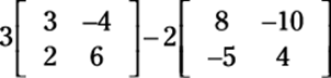
2. Multiply the scalars into the matrices.

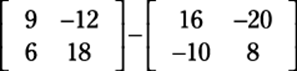
3. Complete the problem by adding or subtracting the matrices.

After subtracting, here is your final answer:

Multiplying matrices by each other

Multiplying matrices is very useful when solving systems of equations because you can multiply a matrix by its inverse (don’t worry, we’ll tell you how to find that) on both sides of the equal sign to eventually get the variable matrix on one side and the solution to the system on the other.

Multiplying two matrices together is not as simple as multiplying the corresponding terms (although we wish it were!). Each element of each matrix gets multiplied by each term of the other at some point.

In fact, multiplication of matrices and dot products of vectors are actually quite similar. Both types of problems have a very methodical way of multiplying certain terms and then adding them together. The difference is that with vectors, this process only needs to be done once. With matrices, you could be here doing this all day, depending on the size of the matrices.

For matrix multiplication, the matrices are written right next to each other with no symbol in between. If you want to multiply matrices AB, the number of columns in A must match the number of rows in B. Each element in the first row of A is multiplied by each corresponding element from the first column of B, and then all of these products are added together to give you the element in the first row, first column of AB. To find the value in the first row, second column position, multiply each element in the first row of A by each element in the second column of B and then add them all together. In the end, after all the multiplication and addition are finished, your new matrix should have the same number of rows as A and the same number of columns as B.

For example, to multiply a matrix with 3 rows and 2 columns by a matrix with 2 rows and 4 columns, you multiply the first row with each of the columns, producing 4 terms in the new row. Multiplying the second row with the columns produces a row of another 4 terms. And the same goes for the last row. You end up with a matrix of 3 rows and 4 columns.

If matrix A has dimensions m x n and matrix B has dimensions n x p, AB is an m-x-p matrix. See Figure 13-4 for a visual representation of matrix multiplication.

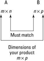
When you multiply matrices, you don’t multiply the corresponding parts like when you add or subtract. You don’t multiply the first row, first column term of the first matrix by the first row, first column term of the second matrix. Also, in matrix multiplication, AB doesn’t equal BA. In fact, just because you can multiply A by B doesn’t even mean you can multiply B by A. The columns in A may be equal to the rows in B, but the columns in B may not equal the rows in A. For example, you can multiply a matrix with 3 rows and 2 columns by a matrix with 2 rows and 4 columns. However, you can’t do the multiplication the other way because you can’t multiply a matrix with 2 rows and 4 columns by a matrix with 3 rows and 2 columns. If you tried to multiply the correct terms together and then add them, somewhere along the way you would run out!

Also note that AB isn’t the same as A × B when it comes to matrices. Two matrices written right next to each other without any symbols in between represent matrix multiplication. The multiplication dot (·) is reserved for scalar multiplication (discussed in “Applying basic operations to matrices”). The symbol × is used to symbolize the cross product, and it represents something completely different. Cross products are only used in 3-x-3 matrices and have certain applications to physics. Because of their specific nature, we do not cover them in this book.

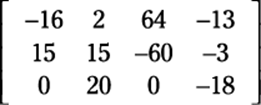
Time for an example of matrix multiplication. Say a problem asks you to multiply the following two matrices:

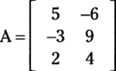
First, check to make sure that you can multiply the two matrices. Matrix A is 3 x 2 and B is 2 x 4, so you can multiply them to get a 3-x-4 matrix as an answer. Now you can proceed to multiply every row of the first matrix times every column of the second.

We lay out this process for you in Figure 13-5. You can start by multiplying each term in the first row of A by the sequential terms in the columns of matrix B. Note that multiplying row one by column one and adding them together gives you row one, column one’s answer. Similarly, multiplying row two by column three gives you row two, column three’s answer.

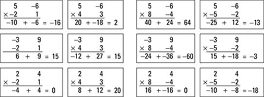
Taking out all the fluff, the answer matrix is

Simplifying Matrices to Ease the Solving Process

In a system of linear equations, where each equation is in the form Ax + By + Cz + . . . = K, the coefficients of this system can be represented in a matrix, called the coefficient matrix. If all the variables line up with one another vertically, then the first column of the coefficient matrix is dedicated to all the coefficients of the first variable, the second row is for the second variable, and so on. Each row then represents the coefficients to each variable in order as they appear in the system of equations. Through a couple of different processes, you can manipulate the coefficient matrix in order to make the solutions easier to find.

Solving a system of equations using a matrix is a great method, especially for larger systems (with more variables and more equations). But don’t get us wrong, these methods work for systems of all sizes, so you have to choose which method is appropriate for which problem. The following sections break down the available simplifying processes.

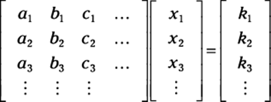
Writing a system in matrix form

You can write any system of equations as a matrix. Take a look at the following system:

To express this system in matrix form, you follow three simple steps:

1. Write all the coefficients in one matrix first (this is called a coefficient matrix).

2. Multiply this matrix with the variables of the system set up in another matrix (some books call this the variable matrix).

3. Insert the answers on the other side of the equal sign in another matrix (some books call this the answer matrix).

The setup appears as follows:

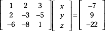
Notice that the coefficients in the matrix go in order — you see a column for x, y, and z.

Finding reduced row echelon form

You can find the reduced row echelon form of a matrix to find the solutions to a system of equations. This process, however, is complicated, and we don’t really recommend it. But just like with completing the square in Chapter 4, sometimes you’ll be required to solve problems in a specific manner, so we help you through the process in this section.

Seeing what’s so great about reduced row echelon form

Putting a matrix into reduced row echelon form is beneficial because this form of a matrix is unique to each matrix (and that unique matrix could give you the solutions to your system of equations).

Two different matrices can’t have the same reduced row echelon form. However, many matrices in row echelon form (not reduced) can be the same; they will all be scalar multiples of one another.

Reduced row echelon form shows a matrix with a very specific set of requirements. These requirements pertain to where any rows of all 0s lie as well as what the first number in any row is. Note: The first number in a row of a matrix that is not 0 is called the leading coefficient. To be considered to be in reduced row echelon form, a matrix must meet all the following requirements:

All rows containing all 0s are at the bottom of the matrix.

All leading coefficients are 1.

Any element above or below a leading coefficient is 0.

The leading coefficient of any row is always to the left of the leading coefficient below it.

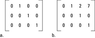
Figure 13-6a shows you a matrix in reduced row echelon form, and Figure 13-6b is not in reduced row echelon form because the 7 is directly above the leading coefficient of the last row and the 2 is above the leading coefficient in row two.

Setting up row echelon form

The row echelon form of a matrix comes in handy for solving systems of equations that are 4 x 4 or larger, because the method of elimination would entail an enormous amount of work on your part. Here we show you how to get a matrix into row echelon form using elementary row operations. These operations are different from the operations on matrices discussed in the previous section because these operations are only carried out on one row of a matrix at a time. You can use any of these operations to get a matrix into reduced row echelon form:

Multiply each element in a single row by a constant.

Interchange two rows.

Add two rows together.

Using these elementary row operations, you can rewrite any matrix so that the solutions to the system that the matrix represents become apparent. We’ll show you how in a bit in the section called “Conquering Matrices.”

Use the reduced row echelon form only if you’re specifically told to do so by a pre-calc teacher or textbook. Otherwise, use any of the other methods we tell you about in this chapter. Reduced row echelon form takes a lot of time, energy, and precision. It can take a lot of steps, which means that you can get mixed up in tons of places. If you have the choice, we recommend opting for a less rigorous tactic (unless, of course, you’re trying to show off).

Putting reduced row echelon form to work with the identity matrix

Perhaps the most famous (and useful) matrix in pre-calculus is the identity matrix, which has 1s along the diagonal from the upper-left corner to the lower-right and has 0s everywhere else. It is a square matrix in reduced row echelon form and stands for the identity element of multiplication in the world of matrices (remember the identity property of multiplication from Algebra II?), meaning that multiplying a matrix by the identity results in the same matrix.

The identity matrix is an important idea in solving systems because if you can manipulate the coefficient matrix to look like the identity matrix (using legal matrix operations, which we tell you about in the previous section), then the solution to the system is on the other side of the equal sign.

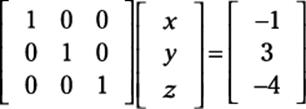
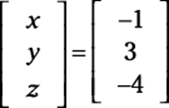
Rewriting this matrix as a system produces the values x = –1, y = 3, and z = –4. But you don’t have to take the coefficient matrix this far just to get a solution. You can write it in row echelon form, as follows:

This setup is different from reduced row echelon form because row echelon form allows numbers to be above the leading coefficients but not below.

Rewriting this system gives you the following from the rows:

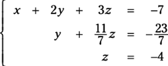
How do you get to the solution — the values of x, y, and z — from there? The answer to that question is back solving, also known as back substitution. If a matrix is written in row echelon form, then the variable on the bottom row has been solved for (as z is here). You can plug this value into the equation above to solve for another variable and continue this process, moving your way up (or backward) until you have solved for all the variables. As with a system of equations, you move from the simplest equation to the most complicated.

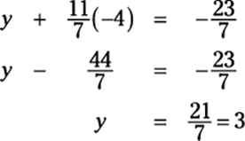
Here’s how you execute the back solving: Now that you know z = –4, you can substitute that value into the second equation to get y:

And now that you know z and y, you can go back further into the first equation to get x:

x + 2(3) + 3(–4) = –7

x + 6 – 12 = –7

x – 6 = –7

x = –1

Augmented form

An alternative to writing a matrix in row echelon or reduced row echelon form is what’s known as augmented form, where the coefficient matrix and the solution matrix are written in the same matrix, separated in each row by colons. This setup makes using elementary row operations to solve a matrix much simpler because you only have one matrix on your plate at a time (as opposed to three!).

Mathematicians are a very lazy bunch, and they like to write as little as possible. Using augmented form cuts down on the amount that you have to write. And when you’re attempting to solve a system of equations that requires many steps, you’ll be thankful to be writing less! Then you can use elementary row operations just as before to get the solution to your system.

Consider this matrix equation:

Written in augmented form, it looks like this:

In the next section you find out how to perform row operations on this augmented matrix, just like a 4-x-3 matrix. You reduce the 3-x-3 coefficient matrix on the left side of column with : entries to reduced row echelon form and obtain the solution naturally.

Conquering Matrices

When you’re comfortable with changing the appearances of matrices (to get them into augmented and reduced row echelon, form, for instance), you are ready to tackle matrices and really start solving difficult systems. Hopefully, for really large systems (four or more variables) you’ll have the aid of a graphing calculator. Computer programs can also be very helpful with matrices and can solve systems of equations in a variety of ways. The three ways we introduce to you in this section are Gaussian elimination, matrix inverses, and Cramer’s rule.

Gaussian elimination is probably the best method to use if you don’t have a graphing calculator or computer program to help you. If you do have these tools, then you can use either of them to find the inverse of any matrix, and in that case the inverse operation is the best plan. If the system only has two or three variables and you don’t have a graphing calculator to help you, then Cramer’s rule is a good way to go.

The previous section is all about getting the matrices into the form that would make it easy for you to solve. Now we take you one step further, actually solving these messy things. By the time we’re finished with you, you’ll be an expert at solving complicated systems of equations.

Using Gaussian elimination to solve systems

Gaussian elimination requires the use of the elementary row operations from the section “Finding reduced row echelon form.” We use an augmented matrix, because that is most often how you’re asked to solve (and is the easiest way to get to the solutions).

The goals of Gaussian elimination are to make the upper-left corner element a 1, use elementary row operations to get 0s in all positions underneath that first 1, get 1s for leading coefficients in every row diagonally from the upper-left to lower-right corner, and get 0s beneath all leading coefficients. Basically, you eliminate all variables in the last row except for one, all variables except for two in the equation above that one, and so on and so forth to the top equation, which has all the variables. Then you can use back substitution to solve for one variable at a time by plugging the values you know into the equations from the bottom up.

You accomplish this elimination by eliminating the x (or whatever variable comes first) in all equations except for the first one. Then eliminate the second variable in all equations except for the first two. This process continues, eliminating one more variable per line, until only one variable is left in the last line. Then solve for that variable.

Elementary operations for Gaussian elimination are the same as the elementary row operations used on matrices in the previous section. We have stated them again here so that you don’t have to look back.

You can perform three operations on matrices in order to eliminate variables in a system of linear equations:

You can multiply any row by a constant: multiplies row three by –2 to give you a new row three.

You can switch any two rows: swaps rows one and two.

You can add two rows together: adds rows 1 and 2 and writes it in row 2.

You can even perform more than one operation. You can multiply a row by a constant and then add it to another row to change that row. For example, you can multiply row one by 3 and then add that to row two to create a new row two: .

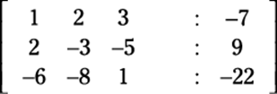
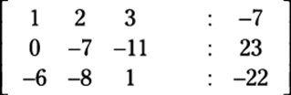
Consider the following augmented matrix:

Now take a look at the goals of Gaussian elimination in order to complete the following steps to solve this matrix:

1. Complete the first goal: to get 1 in the upper-left corner.

You already have it!

2. Complete the second goal: to get 0s underneath the 1 in the first column.

You need to use the combo of two matrix operations together here. Here’s what you should ask: “What do I need to add to row two to make a 2 become a 0?” The answer is –2.

This step can be achieved by multiplying the first row by –2 and adding the resulting row to the second row. In other word, you perform the operation , which produces this new row:

(–2 –4 –6 : 14) + (2 –3 –5 : 9) = (0 –7 –11: 23)

You now have this matrix:

3. In the third row, get a 0 under the 1.

To do this step, you need the operation . With this calculation, you should now have the following matrix:

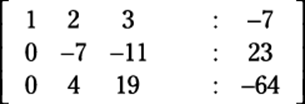
4. Get a 1 in the second row, second column.

To do this step, you need to multiply by a constant; in other words,

multiply row two by the appropriate reciprocal: . This calculation produces a new second row:

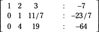
5. Get a 0 under the 1 you created in row two.

Back to the good old combo operation for the third row: . Here’s yet another version of the matrix:

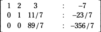
6. Get another 1, this time in the third row, third column.

Multiply the third row by the reciprocal of the coefficient to get a 1:

. You’ve completed the main diagonal after doing the math:

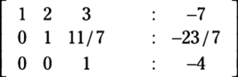
You now have a matrix in row echelon form, which gives you the solutions when you use back substitution (the last row implies that 0x + 0y + 1z = 4, or z = –4). However, if you want to know how to get this matrix into reduced row echelon form to find the solutions, follow these steps:

1. Get a 0 in row two, column three.

Multiplying row three by the constant –11/7 and then adding rows two

and three () gives you the following matrix:

2. Get a 0 in row one, column three.

The operation gives you the following matrix:

3. Get a 0 in row one, column two.

Finally, the operation gives you this matrix:

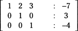
This matrix, in reduced row echelon form, is actually the solution to the system. If you multiply the two matrices on the left side and change the colons back into equal signs, you get a matrix that looks like this:

Multiplying a matrix by its inverse

You can use matrices in yet another way to solve a system of equations. This method is based on the simple idea that if you have a coefficient tied to a variable on one side of an equation, you can multiply by the coefficient’s inverse to make that coefficient go away and leave you with just the variable. For example, if 3x = 12, how would you solve the equation? You’d divide both sides by 3, which is the same thing as multiplying by 1/3, to get x = 4. So it goes with matrices.

In variable form, an inverse function is written as f^–1(x), where f^–1 is the inverse of the function f. You name an inverse matrix similarly; the inverse of matrix A is A^–1. If A, B, and C are matrices in the matrix equation AB = C, and you want to solve for B, how do you do that? Just multiply by the inverse of matrix A, which you write like this:

A^–1[AB] = A^–1C

So the simplified version is B = A^–1C.

Now that you’ve simplified the basic equation, you need to calculate the inverse matrix in order to calculate the answer to the problem.

Finding a matrix’s inverse

First off, we must establish that only square matrices have inverses — in other words, the number of rows must be equal to the number of columns. And even then, not every square matrix has an inverse. If the determinant of a matrix is not 0, then the matrix has an inverse. See the following section on Cramer’s rule for more on determinants.

When a matrix has an inverse, you have several ways to find it, depending how big the matrix is. If the matrix is a 2-x-2 matrix, then you can use a simple formula to find the inverse. However, for anything larger than 2 x 2, we recommend that you use a graphing calculator or computer program (many websites can find matrix inverses for you, and most teachers and textbooks give you the inverse matrix for any system that’s 3 x 3 or bigger).

If you don’t use a graphing calculator, you can augment your original, invertible matrix with the identity matrix and use elementary row operations to get the identity matrix where your original matrix once was. These calculations leave the inverse matrix where you had the identity originally. This process, however, is extremely difficult, and we don’t really recommend it.

With that said, here’s how you find an inverse of a 2-x-2 matrix:

If matrix A is the 2-x-2 matrix , its inverse is as follows:

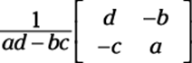
Simply follow this format with any 2-x-2 matrix you’re asked to find.

Using an inverse to solve a system

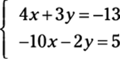
Armed with a system of equations and the knowledge of how to use inverse matrices (see the previous section), you can follow a series of simple steps to arrive at a solution to the system, again using the trusty old matrix. For instance, you can solve the system that follows by using inverse matrices:

These steps show you the way:

1. Write the system as a matrix equation.

When written as a matrix equation (see the earlier section “Writing a system in matrix form”), you get

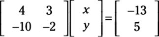
2. Create the inverse matrix out of the matrix equation.

We use this inverse formula:

In this case, a = 4, b = 3, c = –10, and d = –2. Hence ad – bc = 22. Hence, the inverse matrix is

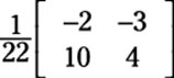
3. Multiply the inverse in the front on both sides of the equation.

You now have the following equation:

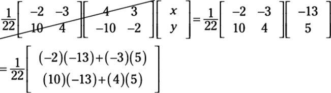
4. Cancel the matrix on the left and multiply the matrices on the right (see the section “Multiplying matrices by each other”).

An inverse matrix times a matrix cancels out. You’re left with

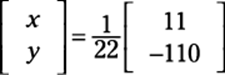
5. Multiply the scalar to solve the system.

You finish with the x and y values:

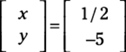
Multiplying the scalar is usually easier after you multiply the two matrices.

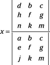
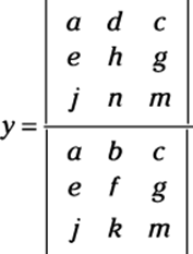
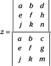
Using determinants: Cramer’s rule

The final method that we show you for solving systems (almost home!) was thought up by Gabriel Cramer and is named after him. As with much of what this chapter covers, a graphing calculator enables you to bypass much of the legwork and has made life a ton easier for pre-calc students. However, if your teacher asks you to use Cramer’s rule, and some certainly will, you can impress him or her with all the know-how you pick up in this section!

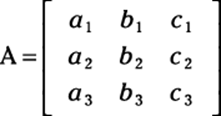
Cramer’s rule says that if the determinant of a coefficient matrix |A| (see the earlier section “Simplifying Matrices to Ease the Solving Process” for more info on how to find the coefficient matrix) is not 0, then the solutions to a system of linear equations can be found as follows:

If the matrix describing the system of equations looks like this:

Then

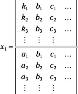
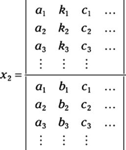
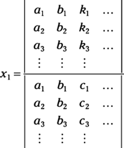
and so on until you have solved for all the variables. In other words, the solution components are readily obtained by computing the appropriate ratios of determinants of a family of matrices. Notice that the denominator of these components is the determinant of the coefficient matrix.

This rule is helpful when the systems are very small or when you can use a graphing calculator to determine the determinants because it helps you find the solutions with minimal places to get mixed up. To use it, you simply find the determinant of the coefficient matrix.

The determinant of a 2-x-2 matrix like this one:

is defined to be ad – bc. The determinant of a 3-x-3 matrix is a bit more complicated. If the matrix is

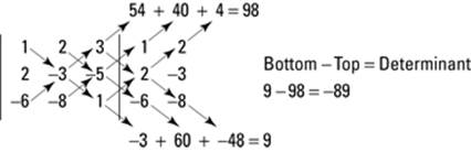
then you can find the determinant by following these steps:

1. Rewrite the first two columns immediately after the third column.

2. Draw three diagonal lines from the upper left to the lower right and three diagonal lines from the lower left to the upper right, as shown in Figure 13-7.

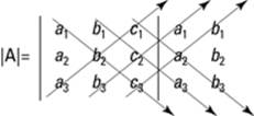
3. Multiply down the three diagonals from left to right, and up the other three.

The determinant of the 3-x-3 matrix is:

To find the determinant of this 3-x-3 matrix:

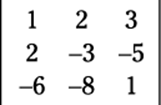
you use a process known as using diagonals, which you can see in Figure 13-8.

After you find the determinant of the coefficient matrix (either by hand or with a technological device), replace the first column of the coefficient matrix with the solution matrix from the other side of the equal sign and find the determinant of that new matrix. Then replace the second column of the coefficient matrix with the solution matrix and find the determinant of that matrix. Continue this process until you have replaced each column and found each new determinant. The values of the respective variables are equal to the determinant of the new matrix (when you replaced the respective column) divided by the determinant of the coefficient matrix.

You can’t use Cramer’s rule when the matrix isn’t square or when the determinant of the coefficient matrix is 0, because you can’t divide by 0. Cramer’s rule is most useful for a 2-x-2 or higher system of linear equations.

To solve a 3-x-3 system of equations such as

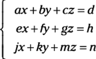
using Cramer’s rule, you set up the variables as follows: