Pre-Calculus For Dummies, 2nd Edition (2012)

Part III. Analytic Geometry and System Solving

Chapter 15. Scouting the Road Ahead to Calculus

In This Chapter

Determining limits graphically, analytically, and algebraically

Pairing limits and operations

Every good thing must come to an end, and for pre-calculus, the end is actually the beginning — the beginning of calculus. Calculus is the study of change and rates of change (not to mention a big change for you!). Before calculus, everything had to be static (stationary or motionless), but calculus shows you that things can be different over time. This branch of mathematics enables you to study how things move, grow, travel, expand, and shrink and helps you do so much more than any other math subject before.

This chapter helps prepare you for calculus by introducing you to the very first bits of the subject. First, we run through the difference between pre-­calculus and calculus. Then we look at limits, which dictate that a graph can get really close to values without ever actually reaching them. Before you get to calculus, math problems always give you a function f(x) and ask you to find the y value at one specific x in the domain (see Chapter 3). But when you get to calc, you look at what happens to the function the closer you get to certain values (like a really tough game of hide-and-seek). Getting even more specific, a function can be discontinuous at a point.

We explore those points one at a time so you can take a really good look at what’s going on in the function at a particular value — that information comes in really handy in calculus when you start studying change. When studying limits and continuity, you’re not working with the study of change specifically, which is why the limit isn’t truly a calc topic — most calc textbooks consider the topics in this chapter to be review material. But after this chapter, you’ll be ready to take the next step.

Scoping Out the Differences between Pre-Calc and Calc

Here are a few basic distinctions between pre-calculus and calculus to illustrate the change in subject:

Pre-calculus: You study the slope of a line.

Calculus: You study the slope of a tangent line to a curve.

A straight line has the same slope all the time. No matter which point you choose to look at, the slope is the same. However, because a curve moves and changes, the slope of the tangent line is different at different points.

Pre-calculus: You study the area of geometric shapes.

Calculus: You study the area under a curve.

In pre-calc, you can rest easy knowing that a geometric shape is always basically the same, so you can find its area with a formula using certain measurements. A curve goes on forever, and depending on which section you’re looking at, its area changes. No more nice, pretty formulas to find area here; instead, you use a process called integration.

Pre-calculus: You study the volume of a geometric solid.

Calculus: You study the volume of complicated shapes called solids of revolution.

The geometric solids you find volume for (prisms, cylinders, and pyramids, for example) have formulas that are always the same, based on the basic shapes of the solids and their dimensions. The only way to find the volume of a solid of revolution, however, is to cut the shape into infinitely small pieces and find the volume of each piece. However, the volume changes over time based on the section of the curve you’re looking at.

Pre-calculus: You study objects moving with constant velocities.

Calculus: You study objects moving with acceleration.

Using algebra, you can find the average rate of change of an object over a certain time interval. Using calculus, you can find the instantaneous rate of change for an object at an exact moment in time.

Pre-calculus: You study functions in terms of x.

Calculus: You study changes to functions in terms of x, with those changes in terms of t.

Graphs of functions generally are referred to as f(x), and you can find those graphs by plotting points. In calculus, you describe the changes to

the graph f(x) by using the variable t, as in .

Our best advice: Calculus is best taken with an open mind and two aspirin! Don’t view it as a bunch of material to memorize. Instead, try to build on your pre-calculus knowledge and experience. Try to glean a deep understanding of why calculus does what it does. In this arena, concepts are key.

Understanding and Communicating about Limits

Not every function is defined at every value of x. Rational functions, for example, are undefined if the denominator of the function is 0. You can use a limit (which, if it exists, represents a value that the function tends to approach as the independent variable approaches a given number) to look at a function to see what it would do if it could. To do so, you take a look at the behavior of the function near the undefined value(s). For example, this function is undefined at x = 3:

You can look at x = 2, x = 2.9, x = 2.99, x = 2.999, and so on. Then you do it again from the other side: x = 4, x = 3.1, x = 3.01, and so on. All these values are defined, except for x = 3.

To express a limit in symbols, you write , which is read as “the limit

as x approaches n of f(x) is L.” L is the limit you’re looking for. For the limit of a function to exist, the left limit and the right limit must both exist and be equivalent:

A left limit starts at a value that’s less than the number x is approaching, and it gets closer and closer from the left-hand side of the graph.

A right limit is the exact opposite; it starts out greater than the number x is approaching and gets closer and closer from the right-hand side.

If, and only if, the left-hand limit equals the right-hand limit can you say that the function has a limit for that particular value of x.

Mathematically, you’d let f be a function and let c and L be real numbers. Then exactly when and . In real-world

language, this setup means that if you took two pencils, one in each hand, and started tracing along the graph of the function in equal measures, the two pencils would have to meet in one spot in the middle in order for the limit to exist. (Looking ahead, Figure 15-1 shows that even though the function isn’t defined at x = 3, the limit exists.)

For functions that are well connected, the pencils always meet eventually in a particular spot (in other words, a limit would always exist). However, you see later that sometimes they do not (see Figure 15-1). The popular unit-step function is defined as f(x) = 0 for x ≤ 0 and f(x) = 1 for x > 0. If you draw this function, you see a unit step jump at x = 0.

Finding the Limit of a Function

You can look for the limit of a function in three ways for a certain value of x: graphically, analytically, and algebraically. We explain how to do it for the sections that follow. However, you may not always be able to reach a conclusion (the function doesn’t approach just one y value at the particular x value you’re looking at). In these cases, the graph jumps and you say it’s not continuous (we cover continuity later in this chapter).

If you’re ever asked to find the limit of a function, and plugging the x value actually works in the function, then most likely you’ve also found the limit. It’s literally that easy!

We recommend using the graphing method only when you’ve been given the graph and asked to find a limit (because graph reading can be very inaccurate, especially if you’re doing the graphing). The analytical method always works for any function, but it’s slow. If you can use the algebraic method, it will save you time. We expand on each method in the sections that follow.

Graphically

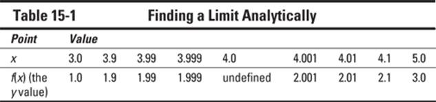
When you’re given the graph of a function and the problem asks you to find the limit, you read values from the graph — something you’ve been doing ever since you learned what a graph was! If you’re looking for a limit from the left, you follow that function from the left-hand side toward the x value in question. Repeat this process from the right to find the right-hand limit. If the y value at the x value is the same from the left as it is from the right (did the pencils meet?), that y value is the limit. Because the process of graphing a function can be long and complicated, we don’t recommend using the graphing approach unless you’ve been given the graph.

For example, in Figure 15-1, find , , and :

: Because the function is defined at x = –1 (which you can see

on the graph because the graph actually has a value — a dot), its limit is the value f(x) = 6 (the y value when x = –1).

: In the graph, you can see a hole in the function at x = 3, which

means that the function is undefined — but that doesn’t mean you can’t

state a limit. If you look at the function’s values from the left — —

and from the right — — you see that the y value gets really close

to 3. So you say that the limit of the function as x approaches 3 is 3.

: You can see that the function has a vertical asymptote at

x = –5 (for more on asymptotes, see Chapter 3). From the left, the function approaches –∞ as it nears x = –5. You can express this mathematically as . From the right, the function approaches ∞ as it nears

x = –5. You write this situation as. Therefore, the limit doesn’t

exist at this value, because one side is –∞ and the other side is ∞.

For a function to have a limit, the left and right values must be the same. A function with a hole in the graph, like , can have a limit, but the func-

tion can’t jump over an asymptote at a value and have a limit (like ).

Analytically

To find a limit analytically, basically you set up a chart and put the number that x is approaching smack dab in the middle of it. Then, coming in from the left in the same row, randomly choose numbers that get closer to the number. Do the same thing coming in from the right. In the next row, you compute the y values that correspond to these values that x is approaching.

Solving analytically is the long way of finding a limit, but sometimes you’ll come across a function (or teacher) that requires this technique, so it’s good for you to know. Basically, if you can use the algebraic technique we describe in the next section, you should. When you can’t, you’re stuck with this method. In typical mathematical style, instructors always teach you the long way before showing you a shortcut. This is why we, too, include the analytic method before the algebraic one. We don’t like to go against the grain; it gives us splinters!

For example, this function is undefined at x = 4 because that value makes the denominator 0:

But you can find the limit of the function as x approaches 4 by using a chart. Table 15-1 shows how to set it up.

The values that you pick for x are completely arbitrary — they can be anything you want. Just make sure they get closer and closer to the value you’re looking for from both directions. The closer you get to the actual x value, though, the closer your limit is as well. If you look at the y values in the chart, you’ll notice that they get closer and closer to 2 from both sides; so 2 is the limit of the function, determined analytically.

You can easily make this chart with a calculator and its table feature. Look in the manual for your particular calculator to discover how. Often you just need to input the function’s equation into “y =” and find a button that says “table.” Handy!

Algebraically

The last way to find a limit is to do it algebraically. When you can use one of the four algebraic techniques we describe in this section, you should. The best place to start is the first technique; if you plug in the value that x is approaching and the answer is undefined, you must move on to the other techniques to simplify so that you can plug in the approached value for x. The following sections break them all down.

Plugging in

The first technique for algebraically solving for a limit is to plug the number that x is approaching into the function. If you get an undefined value (0 in the denominator), you must move on to another technique. But when you do get a value, you’re done; you’ve found your limit! For example, with this method you can find this limit:

The limit is 3, because f(5) = 3.

Factoring

Factoring is the method to try when plugging in fails — especially when any part of the given function is a polynomial expression. (If you’ve forgotten how to factor a polynomial, refer to Chapter 4.)

Say you’re asked to find this limit:

You first try to plug 4 into the function, and you get 0 in the numerator and the denominator, which tells you to move on to the next technique. The quadratic expression in the numerator screams for you to try factoring it. Notice that the numerator of the previous function factors to (x – 4)(x – 2). The x – 4 cancels on the top and the bottom of the fraction. This step leaves you with f(x) = x – 2. You can plug 4 into this function to get 2.

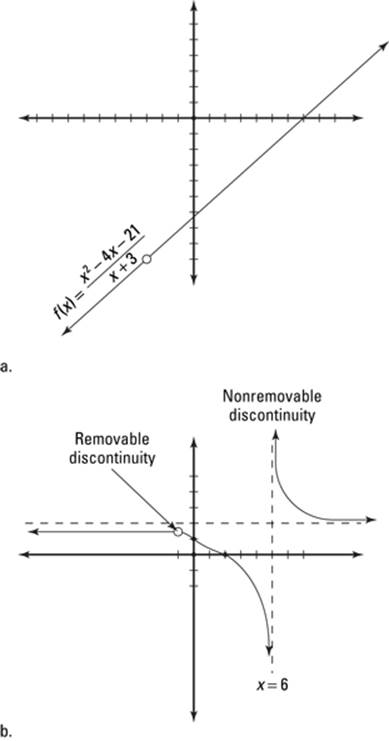
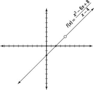
If you graph this function, it looks like the straight line f(x) = x – 2, but it has a hole when x = 4 because the original function is still undefined there (because it creates 0 in the denominator). See Figure 15-2 for an illustration of what we mean.

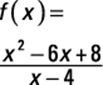If, after you’ve factored the top and bottom of the fraction, a term in the denominator didn’t cancel and the value that you’re looking for is undefined, the limit of the function at that value of x does not exist (which you can write as DNE).

For example, this function factors as shown:

The (x – 7) on the top and bottom cancel. So if you’re asked to find the limit of the function as x approaches 7, you could plug it into the cancelled version and get 11/8. But if you’re looking at the , the limit DNE, because

you’d get 0 on the denominator. This function, therefore, has a limit anywhere except as x approaches –1.

Rationalizing the numerator

The third technique you need to know to find limits algebraically requires you to rationalize the numerator. Functions that require this method have a square root in the numerator and a polynomial expression in the denominator. For example, say you’re asked to find the limit of this function as x approaches 13:

Plugging in numbers fails when you get 0 in the denominator of the fraction. Factoring fails because the equation has no polynomial to factor. In this situation, if you multiply the top by its conjugate, the term in the denominator that was a problem cancels out, and you’ll be able to find the limit:

1. Multiply the top and bottom of the fraction by the conjugate. (See Chapter 2 for more info.)

The conjugate here is . Multiplying through, you get this setup:

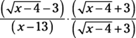
FOIL the tops to get , which simplifies to x – 13 (the middle two terms cancel and you combine like terms from the FOIL).

2. Cancel factors.

Canceling gives you this expression:

The (x – 13) terms cancel, leaving you with this result:

3. Calculate the limits.

When you plug 13 into the function, you get 1/6, which is the limit.

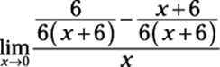
Finding the lowest common denominator

When you’re given a complex rational function, you use the fourth and final algebraic limit-finding technique. The technique of plugging fails, because you end up with a 0 in the denominator somewhere. The function isn’t factorable, and you have no square roots to rationalize. Therefore, you know to move on to the last technique. With this method, you combine the functions by finding the least common denominator (LCD). The terms cancel, at which point you can find the limit.

For example, follow the steps to find the limit:

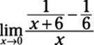
1. Find the LCD of the fractions on the top.

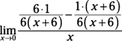
2. Distribute the numerators on the top.

3. Add or subtract the numerators and then cancel terms.

Subtracting the numerators gives you

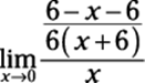
which then cancels to

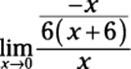
4. Use the rules for fractions to simplify further.

5. Substitute the limit value into this function and simplify.

You want to find the limit as x approaches 0, so the limit here is –1/36.

Operating on Limits: The Limit Laws

If you know the limit laws in calculus, you’ll be able to find limits of all the crazy functions that calc can throw your way. Thanks to limit laws, for instance, you can find the limit of combined functions (addition, subtraction, multiplication, and division of functions, as well as raising them to powers). All you have to be able to do is find the limit of each individual function ­separately.

If you know the limits of two functions (see the previous sections of this chapter), you know the limits of them added, subtracted, multiplied, divided, or raised to a power. If the and , you can use the limit

operations in the following ways:

Addition law:

Subtraction law:

Multiplication law:

Division law: If , then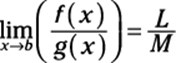

Power law:

The following example makes use of the subtraction, division, and power laws:

If and , you find with the following

calculations:

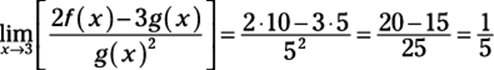
Finding the limit through laws really is that easy!

Exploring Continuity in Functions

The more complicated a function becomes, the more complicated its graph becomes as well. A function can have holes in it, it can jump, or it can have asymptotes, to name a few variations (as you’ve seen in previous examples in this chapter). However, a graph that’s smooth without any holes, jumps, or asymptotes is called continuous. We often say, informally, that you can draw a continuous graph without lifting your pencil from the paper.

All polynomial functions, exponential functions, and logarithmic functions are always continuous at every point (no holes or jumps). If your textbook or teacher asks you to describe the continuity of one of these particular groups of functions, your answer is that it’s always continuous!

Also, if you ever need to find a limit for any of these functions, you can use the plugging in technique we mentioned in the “Algebraically” section because the functions are all defined at every point. You can plug in any number, and the y value will always exist.

You can look at the continuity of a function at a specific x value. You don’t usually look at the continuity of a function as a whole, just at whether it’s continuous at certain points. But even discontinuous functions are only discontinuous at certain spots. In the following sections, we show you how to determine whether a function is continuous. You can use this information to tell whether you’re able to find a derivative (something you’ll get very familiar with in calculus).

Determining whether a function is continuous

Three things have to be true for a function to be continuous at some value x in its domain:

f(c) must be defined. The function must exist at an x value (c), which means you can’t have a hole in the function (such as a 0 in the denominator).

The limit of the function as x approaches the value c must exist. The left and right limits must be the same, in other words, which means the function can’t jump or have an asymptote. The mathematical way to say this is that must exist.

The function’s value and the limit must be the same.

For example, you can show that this function is continuous at x = 4 because of the following facts:

f(4) exists. You can substitute 4 into this function to get an answer: 8.

exists. If you look at the function algebraically (see the earlier

section on this topic), it factors to this:

Nothing cancels, but you can still plug in 4 to get

which is 8.

. Both sides of the equation are 8, so it’s continuous at 4.

If any of the above situations aren’t true, the function is discontinuous at that point.

Dealing with discontinuity

Functions that aren’t continuous at an x value either have a removable ­discontinuity (a hole) or a nonremovable discontinuity (such as a jump or an asymptote):

If the function factors and the bottom term cancels, the discontinuity is removable, so the graph has a hole in it.

For example, this function factors as shown:

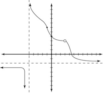
After canceling, it leaves you with x – 7. Therefore x + 3 = 0 (or x = –3) is a removable discontinuity — the graph has a hole, like you see in Figure 15-3a.

If a term doesn’t factor, the discontinuity is nonremovable, and the graph has a vertical asymptote.

The following function factors as shown:

Because the x + 1 cancels, you have a removable discontinuity at x = –1 (you’d see a hole in the graph there, not an asymptote). But the x – 6 didn’t cancel in the denominator, so you have a nonremovable discontinuity at x = 6. This discontinuity creates a vertical asymptote in the graph at x = 6. Figure 15-3b shows the graph of g(x).