Pre-Calculus For Dummies, 2nd Edition (2012)
Part I. Set It Up, Solve It, Graph It
Chapter 5. Exponential and Logarithmic Functions
In This Chapter
![]() Simplifying, solving, and graphing exponential functions
Simplifying, solving, and graphing exponential functions
![]() Checking all the ins and outs of logarithms
Checking all the ins and outs of logarithms
![]() Working through equations with exponents and logs
Working through equations with exponents and logs
![]() Conquering a growth and decay example problem
Conquering a growth and decay example problem
If someone presented you with the choice of taking $1 million right now or taking one penny with the stipulation that the penny would double every day for 30 days, which would you choose? Most people would take the million without even thinking about it, and it would surely surprise them that the other plan is the better offer. Take a look: On the first day, you have only a penny, and you feel like you’ve been duped. But by the last day, you have $5,368,709.12! As you can see, doubling something (in this case, your money) makes it get big pretty fast. This idea is the basic concept behind an exponential function. Bet we have your attention now, don’t we?
In this chapter, we cover two unique types of functions from pre-calc: the exponential and the logarithm. These functions can be graphed, solved, or simplified just like any other function we discuss in this book. We cover all the new rules you need in order to work with these functions; they may take some getting used to, but we break them down into the simplest terms.
That’s great and all, you may be saying, but when will I ever use this complex stuff? (No one in their right mind would offer you the money, anyway.) Well, this chapter’s info on exponential and logarithmic functions will come in handy when working with numbers that grow or shrink (usually with respect to time). Populations usually grow (get larger), whereas the monetary value of objects usually shrinks (gets smaller). You can describe these ideas with exponential functions. In the real world, you can also figure out compounded interest, carbon dating, inflation, and so much more!
Exploring Exponential Functions
 An exponential function is a function with a variable in the exponent. In math terms, you write f(x) = bx, where b is the base and is a positive number. Because 1x = 1 for all x, for the purposes of this chapter we assume b is not 1. If you’ve read Chapter 2, you know all about exponents and their place in math. So what’s the difference between exponents and exponential functions? Prior to now, the variable was always the base — as in g(x) = x2, for example. The exponent always stayed the same. In an exponential function, however, the variable is the exponent and the base stays the same — as in the function f(x) = bx.
The concepts of exponential growth and exponential decay play an important role in biology. Bacteria and viruses especially love to grow exponentially. If one cell of a cold virus gets into your body and then doubles every hour, at the end of one day you’ll have 224 = 16,777,216 of the little bugs moving around inside your body. So the next time you get a cold, just remember to thank (or curse) your old friend, the exponential function.
In this section, we dig deeper to uncover what an exponential function really is and how you can use one to describe the growth or decay of anything that gets bigger or smaller.
Searching the ins and outs of an exponential function
Exponential functions follow all the rules of functions, which we discuss in Chapter 3. But because they also make up their own unique family, they have their own subset of rules. The following list outlines some basic rules that apply to exponential functions:
![]() The parent exponential function f(x) = bx always has a horizontal asymptote at y = 0, except when b = 1. You can’t raise a positive number to any power and get 0 (it also will never become negative). For more on asymptotes, refer to Chapter 3.
The parent exponential function f(x) = bx always has a horizontal asymptote at y = 0, except when b = 1. You can’t raise a positive number to any power and get 0 (it also will never become negative). For more on asymptotes, refer to Chapter 3.
![]() The domain of any exponential function is (–∞, ∞). This rule is true because you can raise a positive number to any power. However, the range of exponential functions reflects that all exponential functions have horizontal asymptotes. All parent exponential functions (except when b = 1) have ranges greater than 0, or (0, ∞).
The domain of any exponential function is (–∞, ∞). This rule is true because you can raise a positive number to any power. However, the range of exponential functions reflects that all exponential functions have horizontal asymptotes. All parent exponential functions (except when b = 1) have ranges greater than 0, or (0, ∞).
![]() The order of operations still governs how you act on the function. When the idea of a vertical transformation (see Chapter 3) applies to an exponential function, most people take the order of operations and throw it out the window. Avoid this mistake. For example, y = 2 · 3x doesn’t become y = 6x. You can’t multiply before you deal with the exponent.
The order of operations still governs how you act on the function. When the idea of a vertical transformation (see Chapter 3) applies to an exponential function, most people take the order of operations and throw it out the window. Avoid this mistake. For example, y = 2 · 3x doesn’t become y = 6x. You can’t multiply before you deal with the exponent.
![]() You can’t have a base that’s negative. For example, y = (–2)x isn’t an equation you have to worry about graphing in pre-calc. If you’re asked to graph y = –2x, don’t fret. You read this as “the opposite of 2 to the x,” which means that (remember the order of operations) you raise 2 to the power first and then multiply by –1. This simple change flips the graph upside down and changes its range to (–∞, 0).
You can’t have a base that’s negative. For example, y = (–2)x isn’t an equation you have to worry about graphing in pre-calc. If you’re asked to graph y = –2x, don’t fret. You read this as “the opposite of 2 to the x,” which means that (remember the order of operations) you raise 2 to the power first and then multiply by –1. This simple change flips the graph upside down and changes its range to (–∞, 0).
![]() Negative exponents take the reciprocal of the number to the positive power. For instance, y = 2–3 doesn’t equal (–2)3 or –23. Raising any number to a negative power takes the reciprocal of the number to the positive power:
Negative exponents take the reciprocal of the number to the positive power. For instance, y = 2–3 doesn’t equal (–2)3 or –23. Raising any number to a negative power takes the reciprocal of the number to the positive power:
![]() , or
, or ![]()
![]() When you multiply monomials with exponents, you add the exponents. For instance, x2 · x3 doesn’t equal x6. If you break down the problem, the function is easier to see: x · x · x · x · x, which is the same as x5.
When you multiply monomials with exponents, you add the exponents. For instance, x2 · x3 doesn’t equal x6. If you break down the problem, the function is easier to see: x · x · x · x · x, which is the same as x5.
![]() When you have multiple factors inside parentheses raised to a power, you raise every single term to that power. For instance, (4x3y5)2 isn’t 4x3y10; it’s 16x6y10.
When you have multiple factors inside parentheses raised to a power, you raise every single term to that power. For instance, (4x3y5)2 isn’t 4x3y10; it’s 16x6y10.
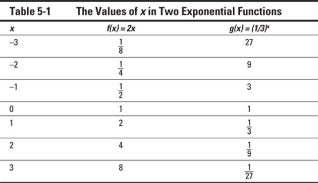
![]() When graphing an exponential function, remember that base numbers greater than 1 always get bigger (or rise) as they move to the right; as they move to the left, they always approach 0 but never actually get there. For example, f(x) = 2x is an exponential function, as is
When graphing an exponential function, remember that base numbers greater than 1 always get bigger (or rise) as they move to the right; as they move to the left, they always approach 0 but never actually get there. For example, f(x) = 2x is an exponential function, as is
![]()
Table 5-1 shows the x and y values of these exponential functions. These parent functions illustrate that, as long as the exponent is positive, a base greater than 1 gets bigger — an example of exponential growth — whereas a fraction (between 0 and 1) gets smaller — an example of exponential decay.
![]() Base numbers that are fractions between 0 and 1 always rise to the left and approach 0 to the right. This rule holds true until you start to transform the parent graphs, which we get to in the next section.
Base numbers that are fractions between 0 and 1 always rise to the left and approach 0 to the right. This rule holds true until you start to transform the parent graphs, which we get to in the next section.
Graphing and transforming an exponential function
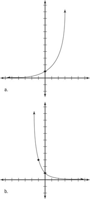
Graphing an exponential function is helpful when you want to visually analyze the function. Doing so allows you to really see the growth or decay of what you’re dealing with. The basic parent graph of any exponential function is f(x) = bx, where b is the base. Figure 5-1a, for instance, shows the graph of
f(x) = 2x, and Figure 5-1b shows ![]() . Using the x and y values from
. Using the x and y values from
Table 5-1, you simply plot the coordinates to get the graphs.
 The parent graph of any exponential function crosses the y-axis at (0, 1), because anything raised to the 0 power is always 1. Some teachers refer to this point as the key point because it’s shared among all exponential parent functions.
Figure 5-1: The graphs of the exponential functions f(x) = 2x and
![]() .
.
Because an exponential function is simply a function, you can transform the parent graph of an exponential function in the same way as any other function (see Chapter 3 for the rules): ![]() , where ais the vertical transformation, h is the horizontal shift, and v is the vertical shift.
, where ais the vertical transformation, h is the horizontal shift, and v is the vertical shift.
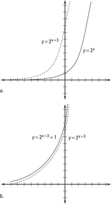
For example, you can graph h(x) = 2(x+3) + 1 by transforming the parent graph of f(x) = 2x. Based on the previous equation, h(x) has been shifted three to the left (h = –3) and shifted one up (v = 1). Figure 5-2 shows each of these as steps: Figure 5-2a is the horizontal transformation, showing the parent function y = 2x as a solid line, and Figure 5-2b is the vertical transformation.
Moving an exponential function up or down moves the horizontal asymptote. The function in Figure 5-2b has a horizontal asymptote at y = 1 (for more info on horizontal asymptotes, see Chapter 3). This change also shifts the range up 1 to (1, ∞).
Figure 5-2: The horizontal transformation (a) and the vertical transformation (b).
Logarithms: The Inverse of Exponential Functions
Almost every function has an inverse. (Chapter 3 discusses what an inverse function is and how to find one.) But this question once stumped mathematicians: What could possibly be the inverse for an exponential function? They couldn’t find one, so they invented one! They defined the inverse of an exponential function to be a logarithm (or log).
A logarithm is an exponent, plain and simple. Recall, for example, that 42 = 16; 4 is called the base and 2 is called the exponent. The logarithm is log4 16 = 2, where 2 is called the logarithm of 16 with base 4. In math, a logarithm is written logb y = x. The b is the base of the log, y is the number you’re taking the log of, and x is the logarithm. So really, the logarithm and exponential forms are saying the same thing in different ways.
Getting a better handle on logarithms
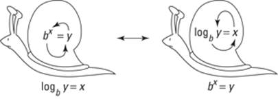
If an exponential function reads bx = y, its inverse, or logarithm, is logb y = x. Notice that the logarithm is the exponent. Figure 5-3 presents a diagram that may help you remember how to change an exponential function to a log and vice versa.
Figure 5-3: The snail rule helps you remember how to change exponentials and logs.
Two types of logarithms are special because you don’t have to write their base (unlike any other kind of log) — it’s simply understood:
![]() Common logarithms: Because the entire number system is in base 10, log y (without a base written) is always meant as log base 10. For example, 103 = 1,000, so log 1,000 = 3. This occurrence is called a common logarithm because it happens so frequently.
Common logarithms: Because the entire number system is in base 10, log y (without a base written) is always meant as log base 10. For example, 103 = 1,000, so log 1,000 = 3. This occurrence is called a common logarithm because it happens so frequently.
![]() Natural logarithms: A logarithm with base e (an important constant in math, roughly equal to 2.718) is called a natural logarithm. The symbol for a natural log is ln. Here’s an example equation: loge y = ln y.
Natural logarithms: A logarithm with base e (an important constant in math, roughly equal to 2.718) is called a natural logarithm. The symbol for a natural log is ln. Here’s an example equation: loge y = ln y.
Managing the properties and identities of logs
You need to know several properties of logs in order to solve equations that contain them. Each of these properties applies to any base, including the common and natural logs (see the previous section):
![]() logb 1 = 0
logb 1 = 0
If you change back to an exponential function, b0 = 1 no matter what the base is. So, it makes sense that logb 1 = 0.
![]() logb x exists only when x ≥ 0
logb x exists only when x ≥ 0
The domain (–∞, ∞) and range (0, ∞) of the original exponential parent function switch places in any inverse function. Therefore, any logarithm parent function has the domain of (0, ∞) and range of (–∞, ∞).
![]() logb bx = x
logb bx = x
You can change this logathrithmic property into an exponential property by using the snail rule: bx = bx. (Refer to Figure 5-3 for an illustration.) No matter what value you put in for b, this equation always works. logb b = 1 no matter what the base is (because it’s really just logb b1).
The fact that you can use any base you want in this equation illustrates how this property works for common and natural logs: log 10x = x and ln ex = x.
![]() blogbx = x
blogbx = x
You can change this equation back to a log to confirm that it works: logb x = logb x.
![]() logb x + logb y = logb(xy)
logb x + logb y = logb(xy)
According to this rule, called the product rule, log4 10 + log4 2 = log4 20.
![]()
![]()
According to this rule, called the quotient rule, ![]() .
.
![]() logb xy = y · logb x
logb xy = y · logb x
According to this rule, called the power rule, log3 x4 = 4 · log3 x.
 Keep the properties of logs straight so you don’t get confused and make a critical mistake. The following list highlights many of the mistakes that people make when it comes to working with logs:
![]() Misusing the product rule:
Misusing the product rule: ![]() ; this equals logb(xy). You can’t add two logs inside of one. Similarly,
; this equals logb(xy). You can’t add two logs inside of one. Similarly, ![]() .
.
![]() Misusing the quotient rule:
Misusing the quotient rule: ![]() ; this equals
; this equals
![]() . Also,
. Also, ![]() .
.
This error messes up the change of base formula (see the following section).
![]() Misusing the power rule:
Misusing the power rule: ![]() ; because the power is on the second variable only. If the formula was written as logb(xy)p, it would equal plogb(xy).
; because the power is on the second variable only. If the formula was written as logb(xy)p, it would equal plogb(xy).
Note: Watch what those exponents are doing. You should split up the multiplication from logb(xyp) first by using the product rule: logb x + logb yp. Only then can you apply the power rule to get logb x + plogb y.
Changing a log’s base
Calculators usually come equipped with only common log or natural log buttons, so you must know what to do when a log has a base your calculator can’t recognize, such as log5 2; the base is 5 in this case. In these situations, you must use the change of base formula to change the base to either base 10 or base e (the decision depends on your personal preference) in order to use the buttons that your calculator does have.
Following is the change of base formula:
![]() ; where m and n are real numbers
; where m and n are real numbers
You can make the new base anything you want (5, 30, or even 3,000) by using the change of base formula, but remember that your goal is to be able to utilize your calculator by using either base 10 or base e to simplify the process. For instance, if you decide that you want to use the common log in the
change of base formula, you find that ![]() . However, if you’re
. However, if you’re
a fan of natural logs, you can go this route: ![]() , which is still 1.465.
, which is still 1.465.
Calculating a number when you know its log: Inverse logs
If you know the logarithm of a number but need to find out what the original number actually was, you must use an inverse logarithm, which is also known as an antilogarithm. If logb y = x, y is the antilogarithm. An inverse logarithm undoes a log (makes it go away) so that you can solve certain log equations. For example, if you know that log x = 0.699, you have to change it back to an exponential (take the inverse log) to solve it: 10log x = 100.699, which simplifies to x = 100.699, so ![]() .
.
You can do this process with natural logs as well. If ln x = 1.099, for instance, then eln x = e1.099, or x = e1.099, so ![]() .
.
The base you use in an antilogarithm depends on the base of the given log. For example, if you’re asked to solve the equation log5 x = 3, you must use base 5 on both sides to get ![]() , which simplifies to x = 53, or x = 125.
, which simplifies to x = 53, or x = 125.
Graphing logs
Want some good news, free of charge? Graphing logs is a snap! You can change any log into an exponential expression, so this step comes first. You then graph the exponential (or its inverse), remembering the rules for transforming (see Chapter 3), and then use the fact that exponentials and logs are inverses to get the graph of the log. The following sections explain these steps for both parent functions and transformed logs.
A parent function
Exponential functions each have a parent function that depends on the base; logarithmic functions also have parent functions for each different base. The parent function for any log is written f(x) = logb x. For example, g(x) = log4 x is a different family than h(x) = log8 x. Here we graph the common log: f(x) = log x.
1. Change the log to an exponential.
Because f(x) and y represent the same thing mathematically, and because dealing with y is easier in this case, you can rewrite the equation as y = log x. The exponential equation of this log is 10y = x.
2. Find the inverse function by switching x and y.
As you discover in Chapter 3, you find the inverse function 10x = y.
3. Graph the inverse function.
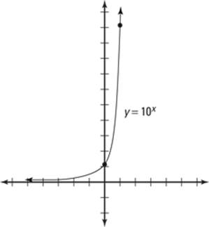
Because you’re now graphing an exponential function, you can plug and chug a few x values to find y values and get points. The graph of 10x = y gets really big, really fast. You can see its graph in Figure 5-4.
Figure 5-4:Graphing the inverse functiony = 10x.
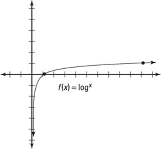
4. Reflect every point on the inverse function graph over the line y = x.
Figure 5-5 illustrates this last step, which yields the parent log’s graph.
Figure 5-5:Graphing the logarithm f(x) = log x.
A transformed log
All transformed logs can be written as f(x) = a · logb(x – h) + v, where a is the vertical stretch or shrink, h is the horizontal shift, and v is the vertical shift.
So if you can find the graph of the parent function logb x, you can transform it. However, we find that most of our students still prefer to change the log function to an exponential one and then graph. The following steps show you how to do just that when graphing f(x) = log3(x – 1) + 2:
1. Get the logarithm by itself.
First, rewrite the equation as y = log3(x – 1) + 2. Then subtract 2 from both sides to get y – 2 = log3(x – 1).
2. Change the log to an exponential expression and find the inverse function.
If y – 2 = log3(x – 1) is the logarithmic function, 3y – 2 = x – 1 is the exponential; the inverse function is 3x – 2 = y – 1 because x and y switch places in the inverse.
3. Solve for the variable not in the exponential of the inverse.
To solve for y in this case, add 1 to both sides to get 3x – 2 + 1 = y.
4. Graph the exponential function.
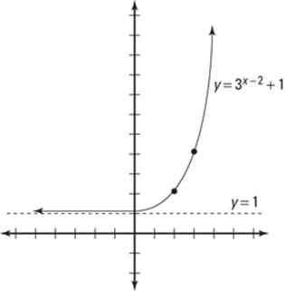
The parent graph of y = 3x transforms right two (x – 2) and up one (+ 1), as shown in Figure 5-6. Its horizontal asymptote is at y = 1 (for more on graphing exponentials, refer to Chapter 3).
Figure 5-6: The transformed exponential function.
5. Swap the domain and range values to get the inverse function.
Switch every x and y value in each point to get the graph of the inverse function. Figure 5-7 shows the graph of the logarithm.
Figure 5-7: You change the domain and range to get the inverse function (log).
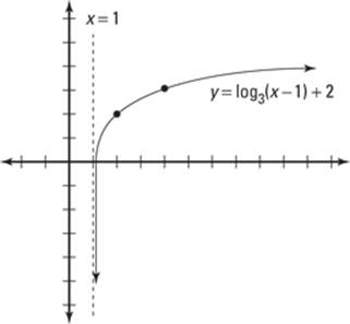
Did you notice that the asymptote for the log changed as well? You now have a vertical asymptote at x = 1. The parent function for any log has a vertical asymptote at x = 0. The function f(x) = log3(x – 1) + 2 is shifted to the right one and up two from its parent function p(x) = log3 x (using transformation rules; see Chapter 3), so the vertical asymptote is now x = 1.
Base Jumping to Simplify and Solve Equations
We’re sure that at some point, your instructor (or boss, perhaps) will ask you to solve an equation with an exponent or a logarithm in it. Have no fear, Pre-Calculus For Dummies is here! You must remember one simple rule, and it’s all about the base: If you can make the base on one side the same as the base on the other, you can use the properties of exponents or logs (see the corresponding sections earlier in this chapter) to simplify the equation. Now you have it made in the shade, because this simplification makes ultimately solving the problem a heck of a lot easier!
In the following sections, you discover how to solve exponential equations with the same base. You also find out how to deal with exponential equations that don’t have the same base. And to round things out, we end with the process of solving logarithmic equations.
Stepping through the process of exponential equation solving
The type of exponential equation you’re asked to solve determines the steps you take to solve it. The following sections break down the types of equations you’ll see, and we give our advice on how to solve them.
The basics: Solving an equation with a variable on one side
The basic type of exponential equation has a variable on only one side and can be written with the same base for each side. For example, if you’re asked to solve 4x – 2 = 64, you follow these steps:
1. Rewrite both sides of the equation so that the bases match.
You know that 64 = 43, so you can say 4x – 2 = 43.
2. Drop the base on both sides and just look at the exponents.
When the bases are equal, the exponents have to be equal. This step gives you the equation x – 2 = 3.
3. Solve the equation.
This example has the solution x = 5.
Getting fancy: Solving when variables appear on both sides
If you must solve an equation with variables on both sides, you have to do a little more work (sorry!). For example, to solve 2x – 5 = 8x – 3, follow these steps:
1. Rewrite all exponential equations so that they have the same base.
This step gives you 2x – 5 = (23)x – 3.
2. Use the properties of exponents to simplify.
A power to a power signifies that you multiply the exponents. Distributing the exponent inside the parentheses, you get 3(x – 3) = 3x – 9, so you have 2x – 5 = 23x – 9.
3. Drop the base on both sides.
The result is x – 5 = 3x – 9.
4. Solve the equation.
Subtract x from both sides to get –5 = 2x – 9. Add 9 to each side to get 4 = 2x. Lastly, divide both sides by 2 to get 2 = x.
Solving when you can’t simplify: Taking the log of both sides
Sometimes you just can’t express both sides as powers of the same base. When facing that problem, you can make the exponent go away by taking the log of both sides. For example, suppose you’re asked to solve 43x – 1 = 11. No integer with the power of 4 gives you 11, so you have to use the following technique:
 1. Take the log of both sides.
You can take any log you want, but remember that you actually need to solve the equation with this log, so we suggest sticking with common or natural logs only (see “Getting a better handle on logarithms” earlier in this chapter for more info).
Using the common log on both sides gives you log 43x –1 = log 11.
2. Use the power rule to drop down the exponent.
This step gives you (3x – 1)log 4 = log 11.
3. Divide the log away to isolate the variable.
You get ![]() .
.
4. Solve for the variable.
Taking the logs gives you ![]() . So
. So ![]() , or
, or ![]() .
.
In the previous problem, you have to use the power rule on only one side of the equation because the variable appeared on only one side. When you have to use the power rule on both sides, the equations can get a little messy. But with persistence, you can figure it out. For example, to solve 52 – x = 33x + 2, follow these steps:
1. Take the log of both sides.
As with the previous problem, we suggest you use either a common log or a natural log. If you use a natural log, you get ln 52 – x = ln 33x + 2.
2. Use the power rule to drop down both exponents.
Don’t forget to include your parentheses! You get (2 – x)ln 5 = (3x + 2)ln 3.
3. Distribute the logs over the inside of the parentheses.
This step gives you 2ln 5 – xln 5 = 3xln 3 + 2ln 3.
4. Isolate the variables on one side and move everything else to the other by adding or subtracting.
You now have 2ln 5 – 2ln 3 = 3xln 3 + xln 5.
5. Factor out the x variable from all the appropriate terms.
That leaves you with 2ln 5 – 2ln 3 = x(3ln 3 + ln 5).
6. Divide the quantity in parentheses from both sides to solve for x.
![]()
Solving logarithm equations
Before solving equations with logs in them, you need to know the following four types of log equations:
![]() Type 1: In this type, the variable you need to solve for is inside the log, with one log on one side of the equation and a constant on the other. Turn the variable inside the log into an exponential equation (which is all about the base, of course). For example, to solve log3 x = –4, change
Type 1: In this type, the variable you need to solve for is inside the log, with one log on one side of the equation and a constant on the other. Turn the variable inside the log into an exponential equation (which is all about the base, of course). For example, to solve log3 x = –4, change
it to the exponential equation 3–4 = x, or ![]() .
.
![]() Type 2: Sometimes the variable you need to solve for is the base. If the base is what you’re looking for, you still change the equation to an exponential equation. If logx 16 = 2, for instance, change it to x2 = 16, in which xequals ±4.
Type 2: Sometimes the variable you need to solve for is the base. If the base is what you’re looking for, you still change the equation to an exponential equation. If logx 16 = 2, for instance, change it to x2 = 16, in which xequals ±4.
Because logs don’t have negative bases, you throw the negative one out the window and say x = 4 only.
![]() Type 3: In this type of log equation, the variable you need to solve for is inside the log, but the equation has more than one log and a constant. Using the rules we present in “Managing the properties and identities of logs,” you can solve equations with more than one log. To solve log2(x – 1) + log2 3 = 5, for instance, first combine the two logs that are adding into one log by using the product rule: log2[(x – 1) · 3] = 5. Turn
Type 3: In this type of log equation, the variable you need to solve for is inside the log, but the equation has more than one log and a constant. Using the rules we present in “Managing the properties and identities of logs,” you can solve equations with more than one log. To solve log2(x – 1) + log2 3 = 5, for instance, first combine the two logs that are adding into one log by using the product rule: log2[(x – 1) · 3] = 5. Turn
this equation into 25 = (x – 1) · 3 to solve it. The solution is ![]() .
.
![]() Type 4: What if the variable you need to solve for is inside the log, and all the terms in the equation involve logs? If all the terms in a problem are logs, they have to have the same base in order for you to solve the equation. You can combine all the logs so that you have one log on the left and one log on the right, and then you can drop the log from both sides. For example, to solve log3(x – 1) – log3(x + 4) = log3 5, first apply the quotient rule to get
Type 4: What if the variable you need to solve for is inside the log, and all the terms in the equation involve logs? If all the terms in a problem are logs, they have to have the same base in order for you to solve the equation. You can combine all the logs so that you have one log on the left and one log on the right, and then you can drop the log from both sides. For example, to solve log3(x – 1) – log3(x + 4) = log3 5, first apply the quotient rule to get
![]()
You can drop the log base 3 from both sides to get
![]()
which you can solve easily by using algebra techniques. When solved, you get
![]()
The number inside a log can never be negative. Plugging this answer back into
part of the original equation gives you ![]() , which is
, which is ![]() . You
. You
don’t even have to look at the rest of the equation. The solution to this equation, therefore, is actually the empty set: no solution.
Always plug your answer to a logarithm equation back into the equation to make sure you get a positive number inside the log (not 0 or a negative number).
Growing Exponentially: Word Problems in the Kitchen
You can use exponential equations in many real-world applications: to predict populations in people or bacteria, to estimate financial values, and even to solve mysteries! Almost every pre-calc textbook includes one section specifically dedicated to exponential word problems, so we do the same here.
Exponential word problems come in many different varieties, but they all follow one simple formula: B(t) = Pert, where
P stands for the initial value of the function — usually referred to as the number of objects whenever t = 0.
t is the time (measured in many different units, so be careful!).
B(t) is the value of how many people, bacteria, money, and so on you have after time t.
r is a constant that describes the rate at which the population is changing. If r is positive, it’s called the growth constant. If r is negative, it’s called the decay constant.
e is the base of the natural logarithm, used for continuous growth or decay.
When solving word problems, remember that if the object grows continuously, then the base of the exponential function can be e.
Take a look at the following sample word problem, which this formula enables you to solve:
Exponential growth exists in your kitchen on daily basis in the form of bacteria. Suppose that you leave your leftover breakfast on the kitchen counter when leaving for work. Assume that 5 bacteria are present on the breakfast at 8:00 a.m., and 50 bacteria are present at 10:00 a.m. Use B(t) = Pert to find out how long it will take for the population of bacteria to grow to 1 million if the growth is continuous.
You need to solve two parts of this problem: First, you need to know the rate at which the bacteria are growing, and then you can use that rate to find the time at which the population of bacteria will reach 1 million. Here are the steps for solving this word problem:
1. Calculate the time that elapsed between the initial reading and the reading at time t.
Two hours elapsed between 8:00 a.m. and 10:00 a.m.
2. Identify the population at time t, the initial population, and the time and plug these values into the formula.
![]()
3. Divide both sides by the initial population to isolate the exponential.
10 = e2r
4. Take the appropriate logarithm of both sides, depending on the base.
In the case of continuous growth, the base is always e: ln 10 = ln e2r
5. Using the power rule (see the section “Managing the properties and identities of logs”), simplify the equation.
ln 10 = 2rln e
ln 10 = 2r
6. Divide by the time to find the rate; use your calculator to find the decimal approximation.
![]() , or
, or ![]() . This rate means that the population is
. This rate means that the population is
growing by more than 115 percent per hour.
7. Plug r back into the original equation and leave t as the variable.
B(t) = 5e1.1513(t)
8. Plug the final amount in B(t) and solve for t, leaving the initial population the same.
1,000,000 = 5e1.1513(t)
9. Divide by the initial population to isolate the exponential.
200,000 = e1.1513(t)
10. Take the log (or ln) of both sides.
ln 200,000 = 1.1513(t)
We recommend not simplifying ln 200,000 at all but rather plugging it into your calculator all as one step. You’ll get less rounding error in the final answer.
11. Divide by the rate on both sides.
10.61 hours = t
Phew, that was quite a workout! One million bacteria in a little more than ten hours is a good reason to refrigerate promptly.