Two-Dimensional Calculus (2011)

Chapter 2. Differentiation

12. Taylor’s theorem; maxima and minima

Let us review the developments since the introduction of the fundamental Lemma 5.1 to see how fundamental this lemma really was. Using it as a basis, we were able to derive in turn the properties of directional derivatives and gradient, the chain rule and its various applications, the mean value theorem, the implicit function theorem, and the Lagrange multiplier method. In our discussion we had assumed only that the functions under consideration were continuously differentiable, and we had not considered the possible existence or behavior of higher order derivatives. As we have seen in Sect. 11, the values of the second derivatives at a point can lead to much more precise information about the nature of a function near that point.

The essence of Lemma 5.1 is that a continuously differentiable function may be approximated near any point by a linear function, and that the coefficients of that linear function are determined by the partial derivatives of the function at the point. The extension of this result, which we wish to prove next, is based on the observation that a linear function is simply a polynomial of first degree. It states that for a function with higher order derivatives one obtains a better approximation by using a polynomial of higher degree, whose coefficients are determined by the higher order derivatives of the function at the point. In precise form, this statement is known as Taylor’s theorem.

We first recall Taylor’s theorem for functions of a single variable.⁸ One form is the following.

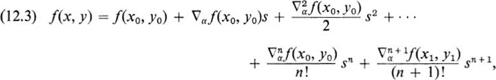
Let f(t) have n + 1 continuous derivatives near t = 0. Then for all sufficiently small t, there is a t₁ between 0 and t such that

For most purposes, the value of Eq. (12.1) is that it represents the function f(t) in the form

where

is a polynomial of degree n, and R_n(t) is a remainder term that tends to zero with t more rapidly than tⁿ; that is, R_n(t)/tⁿ → 0 as t → 0. Conversely, one can show that if f(t) has such a representation, then the coefficients of the polynomial P_n(t) must be given by the successive derivatives of f(t) at t = 0, as in Eq. (12.1).

Suppose now that f(x, y) in a domain D. Given any point (x₀, y₀) in D, let C be the straight line x = x₀ + s cos α, y = y₀ + s sin α. Then we may apply Eq. (12.1) to the function f_c(s):

But the coefficients here are precisely the quantities we introduced in Sect. 11 as higher order directional derivatives. We may therefore rewrite this equation in the form

where (x₁, y₁) is on the line segment between (x₀, y₀) and (x, y).

In many cases, Eq. (12.3), which is no more than Taylor’s theorem for a function of one variable rewritten in different notation, is completely adequate for studying the function f(x, y) near (x₀, y₀). We shall illustrate this later on. First, however, we rewrite Eq. (12.3) in several ways, using the expressions for the various directional derivatives in terms of the partial derivatives of f. By virtue of Eqs. (11.7) and (11.12), we have

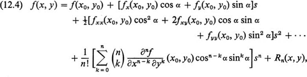
where

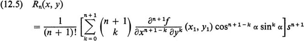
and (x₁, y₁) is on the line joining (x₀, y₀) to (x, y). By the assumption that f , each of the (n + 1)-order partial derivatives of f is continuous, and hence bounded in a circle about (x₀, y₀). Hence

inside a circle about (x₀, y₀).

If we substitute the values

in Eq. (12.4), we obtain the expression

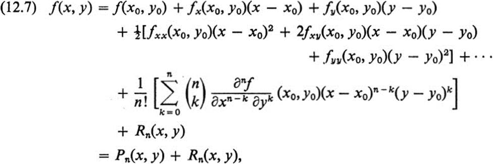
where P_n(x, y) is a polynomial of degree n, and R_n(x, y) satisfies Eq. (12.6). The fact that a function f(x, y) has an expansion of the form of Eq. (12.7) near any point (x₀, y₀) is usually referred to as Taylor’s theorem. Formula (12.7) itself is called the Taylor expansion of f(x, y) through terms of degree n. (See also Ex. 12.14.)

Example 12.1

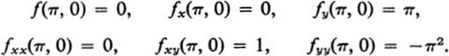
Find the Taylor expansion of the function f(x, y) = sin xy at the point (π, 0) through terms of the second degree.

We have

Hence

By Eq. (12.7),

Remark If we let

then

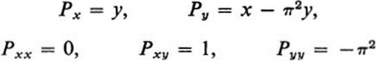
and

Thus in Example 12.1, we have expressed f(x, y) as a polynomial of degree 2 plus a remainder term, and this polynomial has the property that its value at (π, 0) together with the values of its first and second derivatives at that point coincide with the corresponding value of f and its derivatives at (π, 0).

The situation pointed out in the preceding Remark is completely general: the polynomial P_n(x, y) in Taylor’s formula (12.7) is the unique polynomial of degree n whose value and derivatives of degree up to n at (x₀, y₀) coincide with those of f(x, y). This fact may be proved by a direct verification, writing down a general polynomial of degree n, and computing its derivatives of different orders (see Ex. 12.15).

Example 12.2

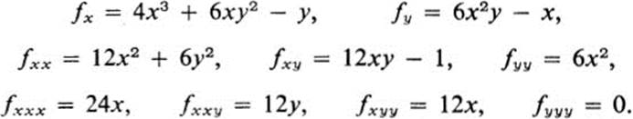
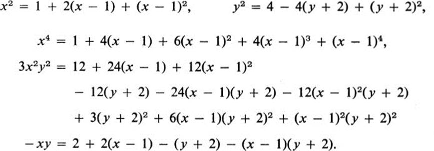
Find the Taylor expansion at the point (1, −2) through terms of degree 3 of the function

Method 1. We find

Substitution in Eq. (12.7) with x₀ = 1, y₀ = −2, and n = 3 yields

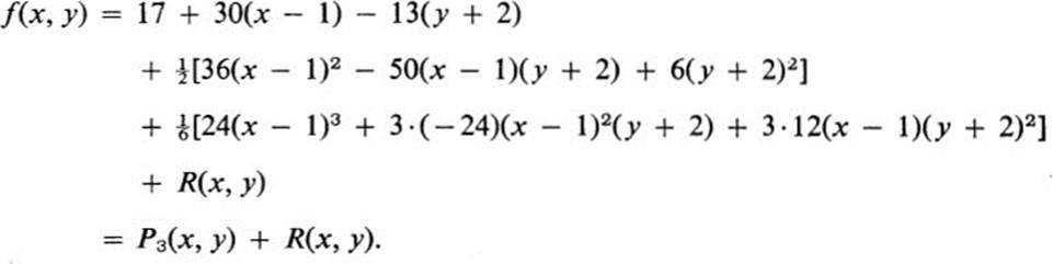
In this case the polynomial P₃(x, y) is much more complicated than the original function, but it also gives a much better description of the behavior of that function near the point (1, −2). Thus, the linear terms in P₃(x, y) give the equation of the tangent plane to the surface z = f(x, y) at (1, −2) and the quadratic terms determine the relative position of the surface and its tangent plane (see Th. 12.1). Actually we can write down the remainder term R(x, y) explicitly, since it is the difference of two polynomials, f(x, y) − P₃(x, y).

In fact, whenever f(x, y) is a polynomial, we can find its Taylor expansion, including the remainder term, much more quickly by purely algebraic methods. We illustrate the procedure as follows.

Method 2. Setting

we have

Thus

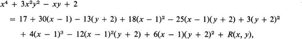
where we have written down all the terms of degree up to 3, which constitute the polynomial P₃(x, y), while the remaining terms give

Note that this remainder term satisfies Eq. (12.6) with n = 3, and one can prove (just as we noted following Eq. (12.2) for functions of one variable) that there is a unique polynomial P_n(x, y) of degree n such that the difference R_n(x, y) = f(x, y) − P_n(x, y) satisfies Eq. (12.6).

We now formulate precisely the role of the second partial derivatives in determining the behavior of a function at a point.

Theorem 12.1 Let f(x, y) in a domain D. Suppose that

at a point (x₀, y₀) in D. There are three possibilities.

In case 1−the surface z = f(x, y) lies above its tangent plane at (x₀, y₀) in some neighborhood of (x₀, y₀).

In case 2−the surface lies below the tangent plane.

In case 3−the surface crosses the tangent plane (Fig. 12.1).

PROOF. We first verify that the three cases listed comprise all the possibilities if f_xxf_yy − ≠ 0. Namely, either f_xxf_yy − < 0, which is case 3,

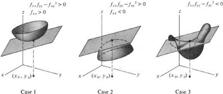
FIGURE 12.1 Position of a surface relative to its tangent plane at a point where f_xxf_yy − ≠ 0 (Cases 1, 2, and 3 of Th. 12.1)

or else f_xxf_yy − > 0. In the latter case it is impossible that f_xx = 0, since that would imply f_xxf_yy − = − ≤ 0. Thus f_xx > 0 or f_xx < 0, which correspond to cases 1 and 2.

We note next that if we introduce the quadratic form

then the three cases in the theorem correspond precisely to

Case 1. Q(X, Y) is positive definite;

Case 2. Q(x, y) is negative definite;

Case 3. Q(x, y) takes on both positive and negative values.

We may write Taylor’s formula (12.7) for f(x, y) in the form

where

and Q(x, y) is defined by Eq. (12.8). Setting

the remainder term R₂(x, y) satisfies, in view of Eq. (12.6),

Note that z = L(x, y) is the equation of the tangent plane to the surface z = f(x, y) at the point (x₀, y₀).

Consider now case 1. Q(x, y) is positive definite, and we have Q(x, y) ≥ λ > 0 for X² + Y² = 1. Then

for all (X, Y) ≠ (0, 0). By Eq. (12.11) we have for some s₀ > 0, that

for s < s₀. Hence

for 0 < s < s₀. But this means

for 0 < s < s₀, which is precisely the statement that z = f(x, y) lies above its tangent plane in a neighborhood of (x₀, y₀).

The same argument works for case 2.

Case 3 is an immediate consequence of Th. 11.2 applied to the function f(x, y) − L(x, y) whose second derivatives coincide with those of f(x, y).

Remark The statement of Th. 12.1 is intuitively obvious if we observe that Q(x, y) = (x₀, y₀)s², so that in case 1, for example, (x₀, y₀) > 0 for all α. This means that the surface z = f(x, y) is concave upwards over every straight line through (x₀, y₀). Similarly, for the other two cases. In fact, this intuitive idea settles case 3 completely, without using Taylor’s theorem. However, it can be deceptive if one wants to use it in cases 1 and 2. Namely, one can have a function f(x, y) with the following property: for each straight line through the origin, f(x, y) ≥ 0 in some interval about the origin, but nevertheless in every neighborhood of the origin, there are points where f(x, y) < 0.

Example 12.3

The function

illustrates the preceding Remark. We have f(0, 0) = 0, and

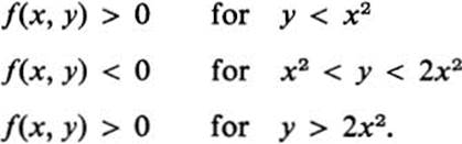
(See Fig. 12.2.) Here the tangent plane to the surface z = f(x, y) at the origin is horizontal. It is simply the x, y plane. For any straight line through the origin, the surface lies above the tangent plane for some interval about the origin. Nevertheless, every neighborhood of the origin contains points where f(x, y) < 0, and at these points the surface lies below the tangent plane.

Example 12.3 is one more illustration of the danger of trying to restrict the study of functions of two variables to properties of the functions along straight lines.

We return now to the question posed at the end of Sect. 6. We observed there that if f(x, y) has a local maximum or minimum at a point (x₀, y₀) and if the gradient of f exists at (x₀, y₀), then

We noted later (after Def. 7.1) that Eq. (12.13) also holds at the summit of a pass.

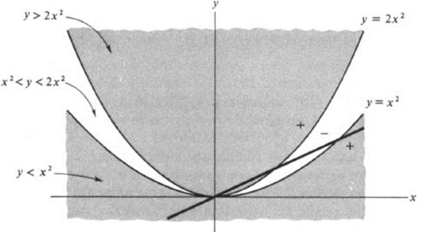
FIGURE 12.2 The set of points where (x² − y)(2x² − y) > 0

Definition 12.1 A point (x₀, y₀) for which Eq. (12.13) holds is called a critical point of the function f(x, y).

The question, then, is to decide whether a given critical point corresponds to a local maximum or a local minimum or neither. The answer is provided in many cases by the following “second-derivative test.”

Theorem 12.2 Let f(x, y) in a domain D, and suppose ∇f(x₀, y₀) = 0. Then at the point (x₀, y₀) we have

Case 1.

f_xxf_yy − > 0, f_xx > 0 ⇒ f has a local minimum;

Case 2.

f_xxf_yy − > 0, f_xx < 0 ⇒ f has a local maximum;

Case 3.

f_xxf_yy − < 0, ⇒ f has a neither a local maximum nor minimum.

PROOF. The condition ∇f(x₀, y₀) = ₀ simply means that the tangent plane to z = f(x, y) is the horizontal plane z = f(x₀, y₀). The result follows immediately from Th. 12.1 (Fig. 12.3).

Remark The name saddle point is sometimes used for a point at which f_xxf_yy − < 0, and it is sometimes used more generally for a point at which the surface crosses the tangent plane. Note that the surface z = x⁴ − y⁴ is “saddle-shaped” at the origin, although f_xxf_yy − = 0 there. Also the

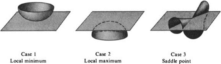
FIGURE 12.3 Picture of a surface z = f(x, y) near a critical point of f(x, y)

function defined by Eq. (12.12) would have a saddle point in the more general sense at the origin. The main fact to observe is that a saddle point in either sense can never be a local maximum or minimum.

When looking for an absolute maximum or minimum of a function of two variables, it is often not necessary to use the second derivative test. One can try to locate all critical points and then find the maximum or minimum value of the function on the critical points.

Example 12.4

Let x, y, z be any three positive numbers whose sum is a fixed number s, that is,

What is the maximum value of the product xyz?

Using Eq. (12.14), we may write the product as a function of two variables:

We are interested in the domain where each factor is positive:

Note that f(x, y) must assume a maximum at some point (x₀, y₀) in the closed set (Fig. 12.4):

But on the boundary of this set f(x, y) = 0, and hence (x₀, y₀) must lie inside the domain D. Since f(x, y) is differentiable throughout D, we conclude that (x₀, y₀) is a critical point of f. But

Since x ≠ 0 and y ≠ 0 in D, at the critical point (x₀, y₀), we must have

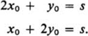
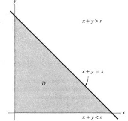
FIGURE 12.4 The set of points: x ≥ 0, y ≥ 0, x + y ≤ s

Solving, we find x₀ = s/3, y₀ = s/3. (In this case we have a single critical point, which must coincide with the absolute maximum.) Thus we have

or in terms of the original problem

We may note that inequality (12.15) has been proved for any three positive numbers. Omitting the middle term, we have

which is called the inequality of the geometric and arithmetic means. (Compare this with inequality (9.2).)

Example 12.5

Find the critical points of the function

and examine the behavior of the function near each point.

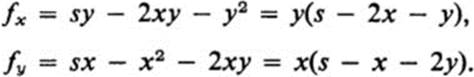
We have

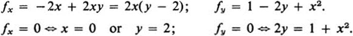
Thus, if x = 0, then y = , and if y = 2, then x² = 1, and x = ± 1. The critical points are therefore (0, ), (1, 2), and (−1, 2). Further

and

Remark It may be observed that no mention is made in Th. 12.2 of the case when f_xxf_yy − = 0. The reason is that in this case the behavior of the function cannot be predicted by the second derivatives alone. The quadratic form (12.8) is then semidefinite, and we might be tempted to think that if it were positive semidefinite the function would still have a local minimum. That would be true, for example, for the function z = x² + y⁴ at the origin, but it is false for z = x² − y⁴, which has the same quadratic terms.

We conclude Chapter 2 by proving a theorem that at first sight may seem to contradict the preceding Remark. The theorem states in effect that even if we cannot predict the behavior of a function at a place where f_xxf_yy − vanishes, we can still describe its over-all behavior in a region where this expression may vanish part of the time. We shall make no further use of this theorem in the present book, and it could easily be omitted on first reading. However, its Corollaries play a fundamental role in many more advanced areas of mathematics, and the proof provides a good illustration of some of the methods developed in this chapter.

Theorem 12.3 Let D be a bounded domain, and let be the set of points in D together with all its boundary points. Let f(x, y) be continuous in , and f(x, y) in D. Suppose that

Then the maximum and minimum values of f in are assumed on the boundary of D.

Remark 1 For simplicity one may picture D to be the interior of the unit circle x² + y² < 1, in which case is the disk x² + y² ≤ 1. This case is sufficient for many applications.

Remark 2 If we had strict inequality in (12.17), then the result would follow immediately from Th. 11.2, since f could not have even a local maximum or minimum in D. The difficulty here is that we allow points where f_xxf_yy − = 0.

PROOF. We give the proof for the maximum. The result follows then for the minimum by considering the function −f.

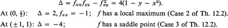
Let M be the maximum value of f(x, y) in , and let m be the maximum on the boundary of D. Clearly m ≤ M, and the assertion of the theorem is that m = M. We proceed by contradiction. Suppose that

Then if (x₀, y₀) is a point in where f(x₀, y₀) = M, (x₀, y₀) cannot lie on the boundary of D, and hence must lie in D itself (Fig. 12.5). We consider next the function

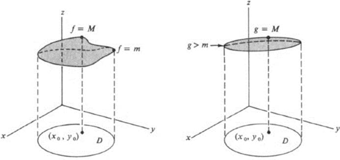
FIGURE 12.5 The surfaces z = f(x, y) and z = g(x, y) in the proof of Th. 12.3

The number is a fixed positive number that is to be chosen sufficiently small so that g(x, y) > m on the boundary of D. That is always possible by (12.18). This means that f(x, y) < g(x, y) on the boundary of D, whereas f(x₀, y₀) = g(x₀, y₀) = M. We introduce the difference

which is continuous in and has a maximum δ at some point (x₁, y₁). Then

and since φ(x, y) < 0 on the boundary of D, (x₁, y₁) must lie somewhere inside D. Since (x₁, y₁) is a maximum of φ(x, y), it is a local maximum along every line through (x₁, y₁), and hence for every α,

But by direct computation from Eq. (12.19) we have

and

Hence,

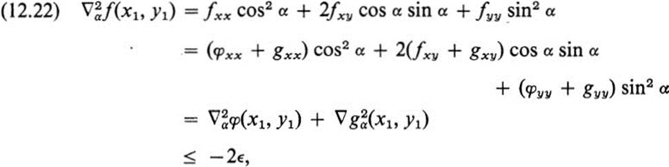
for all α by (12.20) and (12.21). This means that the quadratic form (12.22) is negative definite, and hence, f_xxf_yy − > 0, f_xx < 0 at (x₁, y₁). But this contradicts (12.17). Hence the assumption (12.18) must be false, and the theorem is proved.

Remark The idea of this proof is a simple geometric one. We are trying to prove that if f(x,y) satisfies (12.17) throughout D, then the surface z = f(x, y) cannot protrude over D above its highest point on the boundary of D. If it did, then by choosing a very flat paraboloid, z = g(x, y), which is concave downward, we could lower it until it just touched the surface z = f(x, y) over a point (x₁, y₁) in D. Then the two surfaces would have the same tangent plane at (x₁, y₁), and the surface z = f(x, y) would lie below the surface z = g(x, y). But that would mean that z = f(x, y) was strictly concave downward at (x₁, y₁), which would contradict (12.17).

Corollary 1 If a function f(x, y) satisfies (12.17) in D and is constant on the boundary of D, then it is constant throughout D.

PROOF. If f(x, y) ≡ c on the boundary of D, then for all (x, y) in D we have

Corollary 2 If f(x, y) is harmonic in D, then it assumes its maximum and minimum values on the boundary of D.

PROOF. For a harmonic function f_xx + f_yy = 0, or f_xx = −f_yy, and (12.17) always holds.

Corollary 3 If f(x, y) is harmonic in D and zero on the boundary, then it is zero throughout D.

PROOF. Same as Corollary 1.

Corollary 4 A harmonic function in D is uniquely determined by its values on the boundary of D.

PROOF. Suppose f(x, y) and g(x, y) are both harmonic in D and take on the same value at each boundary point. Then the function φ(x, y) = f(x, y) − g(x, y) is harmonic in D and zero on the boundary of D. By Corollary 3, φ(x, y) ≡ 0, or f(x, y) ≡ g(x, y), in D.

Exercises

12.1 Find all critical points of each of the following functions, and classify them as local maxima, local minima, or saddle points.

a. f(x, y) = 4y³ + x² − 12y² + 36y

b. f(x, y) = x⁴ + y⁴ − 4xy

c. f(x, y) = 2x³ − y³ + 12x² + 27y

d. f(x, y) = (x − 1)(y − 1)(x + y − 1)

12.2 Let f(x, y) be the general quadratic polynomial

a. Show that if AC − B² ≠ 0, then f(x, y) has exactly one critical point.

b. Find the critical point of part a in terms of the coefficients A, B, C, D, E, F.

c. Describe the nature of the critical point in terms of the coefficients.

d. What is the totality of critical points if A, B, and C are all zero?

e. What is the totality of critical points if A, B, and C are not all zero, but if AC − B² = 0?

f. Describe the nature of the critical points in part e in terms of the coefficients. (Hint: see Ex. 10.28.)

12.3 Find the critical points of the following functions, and try to determine whether they are local maxima, local minima, or neither, even in the cases where the “second-derivative test,” Th. 12.2, fails.

a. f(x, y) = x⁶ + y¹⁰

b. f(x, y) = x³ + y³

c. f(x, y) = e^{x2 − y2}

d. f(x, y) = log (2x² − 3xy + 3y² − 10x + 15y + 21)

e. f(x, y) = (x² − y²)²

f. f(x, y) = 2x² − 2 xy + y²

12.4 Show that the function f(x, y) = cos (xe^y) satisfies the equation f_xxf_yy − = 0 at all critical points. (See the discussion of the local maxima and minima of this function at the end of Sect. 6.)

12.5 Let f(x, y) = x³ − 3xy².

a. Show that the origin is the only critical point of this function, and that f_xxf_yy − = 0 at the origin.

b. Describe the surface z = x³ − 3xy² near the origin and explain why it is called a “monkey saddle.” (Hint: see Ex. 3.5e.)

12.6 Show that each of the following functions f(x, y) has a critical point at the origin and try to describe the surface z = f(x, y) in the vicinity of the origin; state, in particular, which functions have a local maximum or minimum at the origin.

a. f(x, y) = x²y²

b. f(x, y) = x³ − y³

c. f(x, y) = x⁴ − x²y² + y⁴

d. f(x, y) = 4x⁴ − 4x²y² + y⁴

e. f(x, y) = x³y − xy³

f. f(x, y) = (2x² − xy + y²)(− x² + 2xy − 3y²

12.7 For each of the following functions find the Taylor expansion through terms of second degree at the points indicated.

a. f(x, y) = 1/(x + 2y) at (1, 1)

b. f(x, y) = sin (x + y) at ( π, 0)

c.

d. f(x, y) = arc cot (x/y) at (0, 1)

12.8 For each of the following functions, find the Taylor expansion through terms of the third degree at the points indicated.

a. f(x, y) = 2x² − xy + 4y − 7, at (1, −2)

b. f(x, y) = x³ − 2x²y + xy² + 4y³ + 7xy − 7, at (0, 0)

c. f(x, y) = x³ − 2x²y + xy² + 4y³ + 7xy − 7, at (1, 0)

d. f(x, y) = x²y² − xy³, at (2, −1)

e. f(x, y) = x²y² − xy³, at (0, 0)

12.9 For each of the following functions find the Taylor expansion through terms of degree n at the points indicated.

a. f(x, y) = e^{x + y}, at (0, 1)

b. f(x, y) = (x + y)ⁿ, at (2, −1)

c. f(x, y) = sin (x + y), at (0, 0)

d. f(x, y) = cos (x + y), at (0, 0)

e. f(x, y) = e^xy, at (0,0) (Hint: see Ex. 11.12e.)

12.10 Let f(x, y) = e^{25 − x2 − y2}.

a. Find the equation of the tangent plane to the surface z = f(x, y) at the point (3, 4), and decide whether the surface lies above or below the tangent plane near that point, or crosses it.

b. Do the same for the point ( , 0).

12.11 Show that the surface z = 3x² − 2xy + 2y² lies entirely above every one of its tangent planes. (Hint: find explicitly the remainder term after expanding through linear terms, and show that it is always positive.)

*12.12 Theorem 12.1 was proved in the text under the assumption that f(x, y) . Actually it is sufficient to assume f(x, y) . For case 3, this is a consequence of Th. 11.2. For cases 1 and 2, it can be shown by noting that the Taylor expansion through linear terms is of the form f(x, y) = L(x, y) + R(x, y), where z = L(x, y) is the equation the tangent plane, and R(x, y) is a quadratic form whose coefficients depend on the values of f_xx, f_xy, f_yy at a point (x₁, y₁) near the given point (x₀, y₀). But for f(x, y) , the functions f_xx and f_xxf_yy - are continuous, so that if they are positive or negative at (x₀, y₀), they have the same sign in some disk about (x₀, y₀). Using these remarks, give a complete proof of Th. 12.1 for f(x, y) . (Note that Ths. 12.2 and 12.3, which are consequences of Th. 12.1, then also follow for f(x, y) .)

12.13 Let f(x, y) near (x₀, y₀) and suppose

Show that

12.14 If we formally define the “product” (∂/∂x)^k(∂/∂y)^l of partial differentiation operators to be ∂^{k + l}/∂x^k ∂y^l, we may write Taylor’s formula in the more compact form:

where

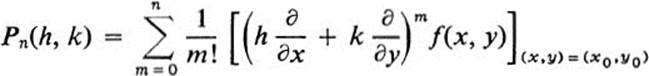
and

where x₁ = x₀ + λh, y₁ = y₀ + λk for some λ, 0 < λ < 1.

Show that by formally using the binomial theorem to expand the expression (h ∂/∂x + k ∂/∂y)ⁿ, applying the corresponding derivatives to f(x, y) and evaluating the result at the point indicated, one obtains Taylor’s formula in the form we have given it. (Note that the final step is to substitute h = x − x₀, k = y − y₀.)

Equivalently, we may write

as a brief (and more easily retained) version of Eq. (11.12).

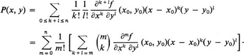
12.15 a. Show that if P(x, y) = Σ C_ij(x − x₀)ⁱ/(y − y₀)^j, then

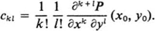
(Hint: see Ex. 11.26.)

b. Show that every polynomial P(x, y) can be written in the form given in part a, where x₀ and y₀ are arbitrary.

(Hint: x^myⁿ = [x₀ + (x − x₀)]^m[y₀ + (y − y₀)]ⁿ.)

c. Show that if f(x, y) and if P(x, y) is a polynomial that has the same value as f(x, y) and the same partial derivatives of all orders up to n at (x₀, y₀), then

Note: a number of problems involve finding the maximum or minimum of a function of three variables subject to a relation between those variables. By using the relation to express one of the variables in terms of the other two, we reduce the problem to a maximum-minimum problem for a function of two variables, which may then be solved by looking for critical points. Exercises 12.16–12.19 are examples.

12.16 Among all rectangular boxes having a given volume V, find the dimensions that require the least material for its construction (that is, the least total surface area).

12.17 Solve Ex. 12.16 for a box without a top.

12.18 If the post office accepts parcels whose total length plus girth does not exceed 60 inches, what dimensions will maximize the volume?

12.19 What is the maximum area of a triangle having a given perimeter p? (Hint: the area A is related to the perimeter p by the formula

where x, y, z are the sides of the triangle, and p = 2s = x + y + z.)

Note that in the preceding four exercises the problem was to find an absolute maximum or minimum of a given function, where the variables are generally restricted by the nature of the problem. (For example, in Ex. 12.19, x ≥ 0, y≥ 0, and z = 2s − x − y ≥ 0, since x, y, and z represent lengths.) A critical approach to these exercises would require specifying the set of points where the function is defined, and verifying first that the extreme value sought does not lie on the boundary of this set of points. (If the function in question satisfied the hypotheses of Th. 12.3, then the extreme value would have to lie on the boundary.) Then assuming that an absolute maximum or minimum exists, it must be taken on at an interior point, and that point must be a critical point of the function. In practice, it is usual to locate a critical point and simply to assume that it provides the answer to the problem. Exercise 12.20 indicates how a careful solution of extremum problems in two variables may be given in a large number of cases.

12.20 For each of the following functions f(x, y), find the absolute maximum and minimum on the given set S. (Note that since in each case S is a closed bounded set and f(x, y) is continuous on S, the function f(x, y) must assume its maximum and minimum somewhere in S. If at an interior point, then the gradient of f must vanish there ; so the first step is to find the value of f(x, y) at each critical point in the interior of S. Next, find the maximum and minimum of f(x, y) on the boundary of S. This amounts to finding the extreme values of f(x, y) along a curve, and may be done by one-variable methods or by using Lagrange multipliers with the precaution that the values of f(x, y) at any possible “corners,” where the boundary curve is not smooth, must be examined also. Note two cases in which the extreme values cannot occur at an interior point, and must occur on the boundary: if ∇f ≠ 0 on S (Lemma 6.1), or if f_xxf_yy − ≤ 0 on S (Th. 12.3).)

a. f(x, y) = x + y, S:x² + y² ≤ 1

b. f(x, y) = x² − 4xy + y², S:x² + y² ≤ 1

c. f(x, y) = x² − 2xy + 2y², S:x² + y² ≤ 1

d. f(x, y) = x⁴ − y⁴, S:x² + y² ≤ 1

e. f(x, y) = (x − 1)² + y², S:x² + y² ≤ 4

f. f(x, y) = (x + 3)² + y², S:x² + y² ≤ 4

g. f(x, y) = x + y, S: − 2 ≤ x ≤ 1, − 1 ≤ y ≤ 3

h. f(x, y) = (x − 2)² + y², S: − 2 ≤ x ≤ 1, − 1 ≤ y ≤ 3

i. f(x, y) = (1 − x²) sin y, S: − 1 ≤ x ≤ 1, − π ≤ y ≤ π

j. f(x, y) = (x² − y²)e^{1 − x2 − y2}, S:x² + y² ≤ 4

k. f(x, y) = (2x² + y²)e^{1 − x2 − y2}, S:x² + y² ≤ 4

12.21 a. Show that if f(x, y) in a domain D, and if f(x, y) has a local minimum at (x₀, y₀), then f_xx ≥ 0, f_yy ≥ 0, and f_xxfy_y − ≥ 0 at (x₀, y₀).

b. What can be said at a local maximum?

12.22 A function f(x, y) is called subharmonic if it satisfies the inequality f_xx + f_yy ≥ 0 in a domain.

a. Show that if f_xx + f_yy > 0 throughout a domain, then f(x, y) cannot have a local maximum.

*b. Using a reasoning analogous to the proof of Th. 12.3, show that if f(x, y) is subharmonic in a bounded domain D and continuous in , then f(x, y) takes on its maximum on the boundary of D. (Hint: if f(x, y) is subharmonic, then

satisfies the hypotheses of part a for every > 0. But if f(x, y) had a larger value at (x₀, y₀) than on the boundary of D, could be chosen sufficiently small so that h(x, y) would have a maximum at an interior point (x₁, y₁) of D, contradicting part a.)

¹ See [14], Section 9.4, or [3], Vol. I, Chapters 7 and 8, concerning the mean-value theorem for one variable.

² A function g(x, y) is called uniformly continuous on a set E, if for every > 0 there exists a δ > 0 such that for every pair of points (x₁, y₁), (x², y²) in E whose distance apart is less than δ, |g(x₁, y₁) − g(x₂, y₂)| < The notion of uniform continuity, although important in certain connections, is not central to the subject matter of this book. A discussion of uniform continuity for functions of two variables may be found in [6], Section 2.3. Theorem 6 of that section is the result quoted in the above remark.

³ See, for example, [3] Vol. I, Section 2.30.

⁴ For proofs of this and related theorems, see [6], Section 2.4.

⁵ The approach used in this section was inspired by the treatment in Chapter 8 of Polya’s book [30]. The reader is referred there for further interesting comments and examples.

⁶ This fact may appear to be intuitively obvious. For a complete proof see [3], Vol. I, Section 8.8.

⁷ See Exercise 26.16. For other proofs, see [29], Section 28, and [31], Chapter 2, Theorem 2. Compare also Corollary 2 of Theorem 12.3. Both that Corollary and the property mentioned here are known as the maximum principle for harmonic functions.

⁸ See, for example, [3], Section 7.6 or [14], Section 9.6.