Two-Dimensional Calculus (2011)

Chapter 3. Transformations

13. Pairs of functions; geometric representation

One of the major lessons learned in Chapter 2 was that for the proper study of a function of two variables it is not sufficient to consider the function with respect to each variable separately. In the present chapter we shall see that when confronted with a pair of functions it is often advantageous to treat the pair as a single entity rather than as two separate functions.

Pairs of functions of two variables appear in many guises. We give the following examples.

Example 13.1

The gradient Given a differentiable function f(x, y), its gradient associates with it a pair of functions ; namely, the partial derivatives f_x(x, y) and f_y(x, y).

Example 13.2

Vector fields Given a domain D, a vector field or vector function on D assigns to each point (x, y) of D a vector v(x, y). This is equivalent to giving a pair of functions in D; namely, the two components of the vector v(x, y). Example 13.1 is a special case of this, in which to each point (x, y) corresponded the gradient vector of f(x, y) at that point. Many other examples arise in physics, such as the gravitational or electromagnetic force fields and the velocity field of a fluid flow.

Example 13.3

Coordinate transformations Under a change of coordinates in the plane, the expressions for the new coordinates of a point in terms of the old constitute a pair of functions. Thus

the relations between rectangular and polar coordinates, express x and y as functions of the two variables r and θ.

Example 13.4

Motions in the plane A motion of the plane into itself, such as a Euclidean motion or a similarity transformation, may be described by assigning to each point (x, y) the point (u, v) to which it is displaced by the motion. Each of the coordinates u, v may then be considered as a function of (x, y). More general motions, such as fluid motion, may be described in the same way, by assigning to each point (x, y) the coordinates of the point it reaches after a given interval of time.

It is important to observe that a single pair of functions may arise in all of these ways. Conversely, a given pair of functions may be interpreted in various ways. Let us illustrate these general remarks with a particular example.

Example 13.5

For a fixed value of a, consider the pair of functions

of x and y.

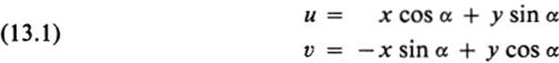
Interpreted as a motion, these equations describe a clockwise rotation of the plane through an angle α (Fig. 13.1). With respect to a fixed coordinate system, we have

(See Sect. 15 for a detailed discussion of rotations.)

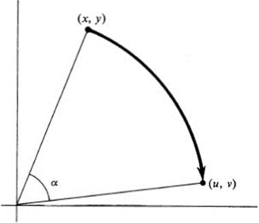
FIGURE 13.1 Rotation through angle α

As a coordinate transformation, Eqs. (13.1) describe the relation between the coordinates (x, y) of a point with respect to one set of axes, and the coordinates (u, v) of the same point with respect to a pair of axes making an angle α with the original pair (Fig. 13.2).

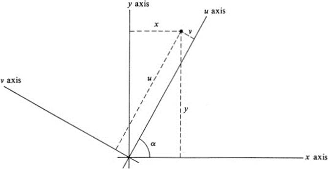
FIGURE 13.2 Rotation of coordinate axes

As a vector field, Eqs. (13.1) assign to each point (x, y) the vector u, υ = x cos α + y sin α,−x sinα +y cos α . We note that

so that the vectors u, υ all have the same length r along the circle x² + y² = r². Furthermore, u, υ makes an angle α with the vector x, y , which is the radius vector to this circle. The vector field is illustrated in Fig. 13.3.

Finally, we may try to find a function f(x, y) such that u, υ = ∇f. However, for the pair of Eqs. (13.1) no such function exists, as we shall see later, by virtue of Lemma 19.1.

We defer further discussion of vector fields until Sect. 19, and of coordinate transformations until Sect. 20. For the greater part of this chapter we shall concentrate on the last of our four interpretations of a pair of functions, the one given in Example 13.4. The word “motion” will be interpreted in its wider sense, and replaced by the term “transformation” or “mapping.” For ease of visualization it is most convenient to picture two separate planes. It is always possible later to consider the two planes as coinciding if we wish to picture a transformation of a plane into itself.

Definition 13.1 A plane transformation or mapping assigns to each point p of a plane domain D, a point q = F(p) of another (or the same) plane. The point q is called the image of p under F (Fig. 13.4).

FIGURE 13.3 Vector field x cos α + y sin α, − x sinα + y cos α

Remark The words “transformation” and “mapping” (or “map”) are used interchangeably throughout most of mathematics, although in certain contexts it is more customary to use one rather than the other.

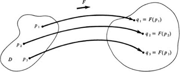
FIGURE 13.4 Plane mapping

The ability to visualize transformations is a skill that may be acquired with practice. It is useful not only in understanding the statement of theorems, but in discovering the underlying idea of their proofs. As an aid in the visualization, it is often useful to consider not only the image of individual points, but of sets of points, such as all points lying on a certain line, or on a certain figure. Then letting the line or figure vary over D, we may picture the way the image varies, and thus obtain an over-all view of the transformation.

In order to describe a transformation analytically, let us denote the coordinates of points in the first plane by (x, y) and those of the second plane by(u, υ). We use the notation

to indicate that the mapping F takes the point (x, y) onto the point (u, υ). The mapping is given explicitly by expressing each of the coordinates u, υ as a function of x and y :

These general statements will be clarified by a number of concrete examples. In these examples the domain D where F is defined consists of the entire x, y plane.

Example 13.6

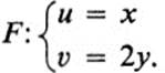
Under this transformation each vertical line x = a maps onto the vertical line u = a with the same abscissa. Each horizontal line y = b maps onto the horizontal line υ = 2b, twice as far from the horizontal axis. Thus F takes the point (a, b) into the point (a, 2b). If the u, υ plane is pictured as coinciding with the x, y plane, then this transformation may be described as a uniform stretching of the plane, by a factor of two, away from the x axis (Fig. 13.5).

Example 13.7

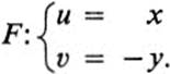
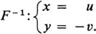
In this case each horizontal line goes into a horizontal line on the opposite side of the axis. If the two planes coincide, these equations define a reflection in the x axis (Fig. 13.6).

Example 13.8

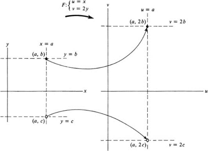
FIGURE 13.5 Map F:(x, y) → (x, 2y)

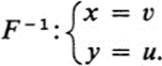
Here each horizontal line goes into a vertical one, and each vertical line into a horizontal one. If the two planes coincide, then all points on the line y = x remain fixed, while all other points are reflected in this line (Fig. 13.7).

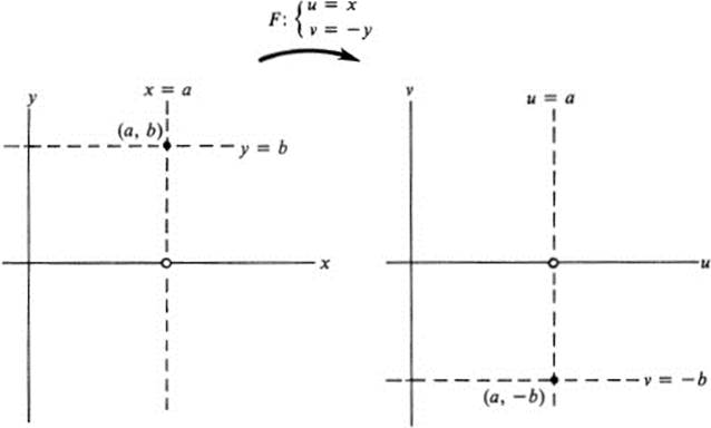
FIGURE 13.6 Map F:(x, y)→(x, −y)

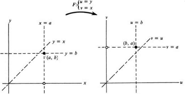
FIGURE 13.7 Map F:(x, y)→(y, x)

Example 13.9

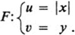
Here we have a new feature. Each pair of vertical lines x = a, x = −a maps onto the same vertical line u = |a|.

All points on the horizontal line y = b map into points of the horizontal line υ = b but in this case we get only half of the line υ = b in our image, because u = | x| ≥ 0. Thus the whole x, y plane maps into the right half of the u, υplane. Each pair of points (a, b), (−a, b) map onto a single point. If the u, υ plane is pictured as coinciding with the x, y plane then this transformation can be described very simply as a “folding over.” We leave the right half plane fixed, and we fold the left half plane along the y axis over onto the right half (Fig. 13.8).

FIGURE 13.8 Map F:(x, y)→(|x|, y)

At this point we interrupt our catalogue of special transformations to make some general definitions.

Definition 13.2 A mapping is called one-to-one or injective if any two distinct points map onto two distinct points. In other words, F is one-to-one if P₁ ≠P₂ implies F(p₁) ≠ F(p₂).

A mapping of a domain D into a domain E is called onto or surjective if every point qof E is the image of some point p.In other words, if to each q in E there exists at least one point p in D such that F(p) = q.

A mapping which is both one-to-one and onto is called bijective.

Note that under a bijective mapping F, each point q of E is the image of one and only one point p. We then have an inverse mapping q → p, defined throughout the domain E, which assigns to each point q in E the unique point psuch that q = F(p).

Definition 13.3 A mapping G is called the inverse of a mapping F if

The standard notation for the inverse mapping of F is F⁻¹ (Fig. 13.9).

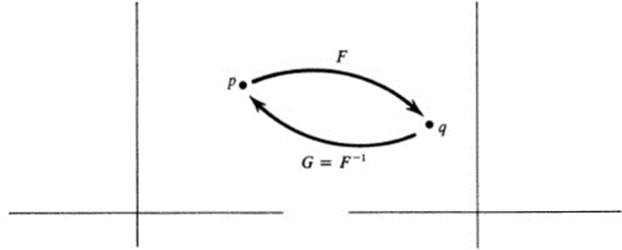
FIGURE 13.9 Inverse map

Remark For the remainder of this section, and also in the next two sections, the domains D and E consist of the entire plane.

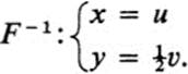
If a mapping is given in coordinates by u = f(x, y), υ = g(x, y),then finding the inverse means solving these equations for x and y in terms of u and υ. In Examples 13.6-13.8, the mappings are all bijective, and it is easy to find the inverse.

Example 13.6a

Example 13.7a

Example 13.8a

However, in Example 13.9, the mapping is neither one-to-one nor onto, since the point (1,0), for example, is the image of two distinct points, (1, 0) and (− 1, 0), while the point (− 1, 0) is not an image at all. Thus, this mapping does not have an inverse.

We now continue our list of examples.

Example 13.10

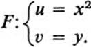
This mapping resembles the one in Example 13.9 in many ways. Each pair of vertical lines x = a, x = − a maps onto a single vertical line u = a² while each horizontal line y = b maps onto the right half of the horizontal line υ = b(Fig. 13.10). However there is a great deal of “distortion,” since vertical lines near the y axis are mapped onto lines still nearer to the u axis, while those far from the y axis are mapped onto lines much further from the υ axis. In some sense, though, this mapping has the same basic properties as the one in Example 13.9. Namely, each point in the right half plane u > 0 is the image of precisely two points in the x, y plane, while points in the left half plane u < 0 are not images at all.

Example 13.11

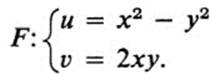
Again we try to visualize this mapping by looking at the horizontal and vertical lines in the x, y plane, and their images in the u, υ plane. Whenever x = a, we have u = a² − y², υ = 2ay, or u = a² − υ²/4a². This is the equation of a parabola in the u, υ plane with vertex at (a², 0), andopening to the left. Similarly, if y = b, then u = x² − b², υ = 2bx, and u = υ²/4b² − b², which is a parabola with vertex (− b², 0), and opening to the right. Note also that the lines x = − a and y = − b map into the same two parabolas as x = a and y = b (Fig. 13.11). It is

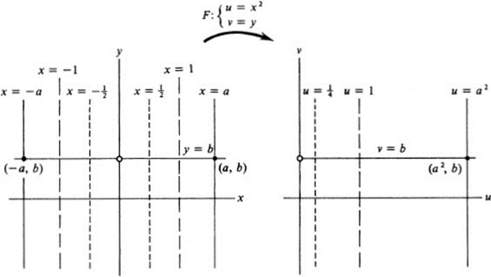
FIGURE 13.10 Map F: (x, y)→ (x², y)

clear that the points (a, b) and (−a, −b) both map into the same point (a² − b², 2ab), while the points (a, −b) and (−a, b) map into the point (a² − b², −2ab).

Although we get some idea of the mapping F in Example 13.11 from the above description, it is certainly not as complete a picture as we were able to form in the previous examples. There are two very useful devices that may

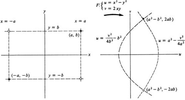
FIGURE 13.11 Map F:(x, y)→(x² − y², 2xy)

aid in many cases in the visualization of a mapping. The first is that of the “inverse image.”

Definition 13.4 The inverse image of a set S under a mapping F is the set of all points p such that F(p) is in S. It is denoted by F^-1(S).

Note that if F has an inverse map, then the inverse image of S is simply the image of S under the inverse map F⁻¹. However, the inverse image of S is a well-defined set of points for any mapping F. In particular, the inverse image of a point q consists of all points p that map into q under F.

Now it is often advantageous, when studying a particular map F, to look at the inverse image of lines in the u, υ plane. Note that the inverse image of a vertical line u = c, is no more nor less than a level curve of the function u(x, y). For the mapping of Example 13.11, the inverse image of u = c is the curve x² −y² = c, which is a rectangular hyperbola. Similarly, the inverse image of the horizontal line v = d is the curve 2xy = d. The intersection of these two curves gives the inverse image of the point (c, d) (Fig. 13.12). See Exercise 13.9 for a more detailed analysis of Example 13.11 by the method of inverse images.

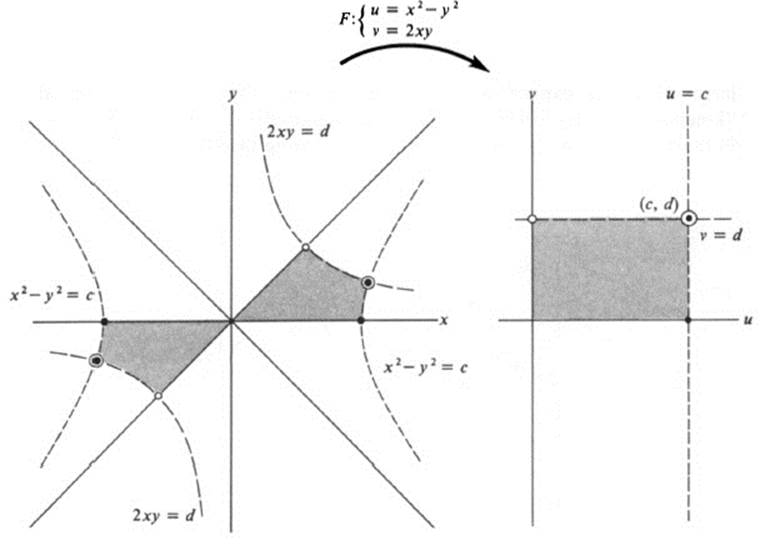
FIGURE 13.12Map F:(x,y)→(x²−y², 2xy); inverse images

We may note that as a general rule it is much easier to construct inverse images than “forward images,” because the former are directly given as a relation between x and y, whereas the latter involve a parameter that must be eliminated to get a relation between u and υ.

The second device, which turns out to be the more useful in this case, is the introduction of polar coordinates. Just as in several of the examples in Sect. 3, the fact that we are dealing with homogeneous polynomials is particularly suggestive of this approach. Let us use r, θ for polar coordinates in the x, y plane, and R, φ in the u, υ plane. Then

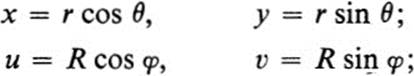
and

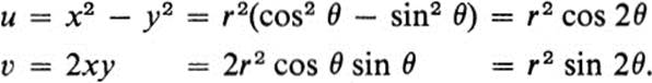
Thus the mapping F may be described in polar coordinates by

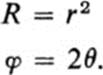
Each circle x² + y² = maps onto the circle u² + υ² = R = whose radius is the square of the original radius. Each ray θ = θ₁ maps onto the ray φ = 2θ₁(Fig. 13.13). It is now easy to visualize the total behavior of this map. Small circles about the origin are contracted into smaller circles, while large circles are expanded into still larger ones. One may give a good “kinematic” description by observing that as a ray θ = c rotates once around in the positive direction, its image is a ray rotating twice as fast, and going

FIGURE 13.13Map F:(x, y) → (x²−y², 2xy); polar coordinates

twice around in the positive direction. Incidentally, although it was clear from our first description that this map is not one-to-one, it was not obvious that every point in the u, υ plane was the image of some point in the x, y plane. However, we now see that the origin in the u, υ plane corresponds precisely to the origin the x, y plane, while every other point in the u, υ plane is the image of exactly two points in the x, y plane. This map is therefore surjective.

Exercises

13.1 Try to visualize each of the following transformations. Make a sketch, and describe the transformation in words.

a.

b.

c.

d.

e.

f.

g.

h.

i.

j.

k.

l.

m.

13.2 For each of the following transformations, introduce polar coordinates r, θ in the x, y plane and R, φ in the u, υ plane ; express R and φ as functions of r, θ, and use these expressions to describe the transformation geometrically as in Example 13.11.

a.

b.

c.

d.

e.

f.

g.

*h.

13.3 A transformation of the type

where b is a nonzero constant, is called a “shear transformation.”

a. Draw the horizontal line segments 0 ≤ x ≤ 1, y = c for c = 0, c = and c = , and draw their images under the transformation F. (Consider separately the cases b > 0 and b < 0.)

b. Draw the inverse images of the line segments 0 ≤ u ≤ 1, υ = c, where c = 0, , 1. (Consider again b > 0 and b < 0.)

c. Find the inverse of a shear transformation, and show that it is also a shear transformation.

13.4 For each of the following transformations F, find the inverse transformation F⁻¹.

a.

b.

c.

d.

e.

f.

13.5 Classify each of the following transformations as injective, surjective, bijective, or none of these. Explain your answer.

a.

b.

c.

d.

e.

f.

g.

h.

i.

j.

13.6 In each of the following transformations, find the inverse image of the u axis.

a.

b.

c.

d.

13.7For each of the transformations in Ex.13.6, find the inverse image of the line υ = u

13.8 For each of the following transformations, find the inverse image of the circle u² + υ² = R².

a.

b.

c.

d.

e.

f.

g.

h.

13.9 Study the transformation u = x² − y², υ = 2xy by a detailed use of inverse images. Carry out the following steps.

a. What is the inverse image of the u axis?

b. What is the inverse image of the υ axis?

c. Describe the inverse image of the horizontal line v = d for the two cases d > 0 and d < 0.

d. Describe the inverse image of the vertical line u = c for the two cases c > 0 and c < 0.

e. Describe the way the curves in part d vary as the line u = c moves to the right, starting with the υ axis.

f. Copy Fig. 13.12. Note that the u, υ plane is divided into nine parts by the lines u = 0, u = c, v = 0, υ = d, and that the x, y plane is divided into eighteen parts by the inverse images of these lines. Number the nine parts in the u, υ plane, and place the corresponding number in the inverse image of each of these parts.

Note: seeing how the inverse images of the different parts “fit together” is a useful device in many cases for obtaining an over-all picture of a given transformation.

13.10 Consider the transformation

a. Introduce polar coordinates R, φ in the u, υ plane and express R and φ as functions of x, y.

b. What is the inverse image of a circle u² + υ² = R²?

c. If a point moves upward along a vertical line x = c, describe the motion of the image point in the u, υ plane.

d. What is the image of the x axis?

e. What is the image of the line y = π?

f.What is the image of the line y = π?

g. What is the image of the line y = 2π?

h. If a point moves from left to right along a horizontal line y = d, describe the motion of the image point in the u, υ plane.

i. Picture the line y = d moving upward, and describe the way the image of this line varies in the u, υ plane.

j. Is this transformation surjective? Explain.

13.11 Consider the transformation

a.If p is the point (−1, 1), what is F(p)?

b. If p is the point (−1, 1), show that F⁻¹(F(p)) ≠ p.

c. Find a set S of points in the u, υ plane such that the image under F of the set F⁻¹(S) does not coincide with S.

13.12 Let F be a transformation of a domain D into a domain E.

a. Show that F is injective if and only if there exists a transformation G of E into D satisfying G(F(p)) = p for all p in D.

b. Show that F is surjective if and only if there exists a transformation G of E into D satisfying F(G(q)) = q for all q in E.

c. Show that F is bijective if and only if there exists a transformation G of E into D satisfying both G(F(p)) = p for all p in D and F(G(q)) = q for all q in E; show that this transformation G is F⁻¹.

Note: the fact that D and E are plane domains is irrelevant in Ex. 13.12. The three parts hold without change if F is a mapping of any set D into any set E. The transformation G defined in part a is called a left inverse of F and the transformation G of part b is called a right inverse of F. Thus Ex. 13.12 may be summed up as follows: F has a left inverse ⇔ F is injective ⇔ F has a right inverse ⇔ F is surjective; F has an inverse F has a simultaneous left and right inverse ⇔ F is bijective.

13.13 If F is a mapping of a domain D into a domain E, the image of the domain D is called the range of F. In other words, the range of F is the set S of points q in E such that q = F(p) for some p in D. Thus F is surjective ⇔ S = E. It is always possible to consider F as a mapping of D into S. If F is injective, it will have an inverse when considered as a map of D into the range S.

For each of the following mappings, find the range S. If the mapping is injective, find the inverse mapping defined on the range.

a.

b.

c.

d.

e.

f.

g.

(Note:use principal value of arc tan.)

13.14 In many cases the simplest way to show that a given transformation F:u = f(x, y), υ = g(x, y) is bijective is to solve explicitly for x and y as functions of u and υ. Consider, for example, the transformation

a. Solve these equations for x and y as functions of u and v.

b. Explain carefully why your solution demonstrates that the image of the x, y plane is the entire u, υ plane.

c. Explain carefully why the solution implies that two different points in the x, y plane cannot have the same image in the u, υ plane.