Two-Dimensional Calculus (2011)
Chapter 3. Transformations
16. Differentiable transformations
Having studied a few special transformations in some detail, we now examine more general transformations.
Definition 16.1A transformation
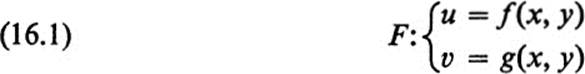
defind in a domain D is of class ![]() in D if f(x, y)∈
in D if f(x, y)∈![]() and g(x, y)∈
and g(x, y)∈ ![]() in D.
in D.
By a differentiable transformation we mean a transformation that is of class ![]() for some k ≥ 1.
for some k ≥ 1.
Examples 13.6-13.11 were all differentiable transformations with the exception of Example 13.9. (The function u = |x| is not differentiable at x = 0.) In all those examples the domain D was the entire plane. If we set
we obtain a transformation of class ![]() in the domain D:x2 + y2 < 1.
in the domain D:x2 + y2 < 1.
As in our study of a single function of two variables, we start our investigation of a pair of functions by asking what happens along an arbitrary curve C in the domain D. We use our standard notation
![]()
where x(t) and y(t) are continuously differentiable functions for a ≤ t ≤ b. The image of the curve C under the transformation F is a curve Γ in the u, υ plane :

(Figure 16.1.)
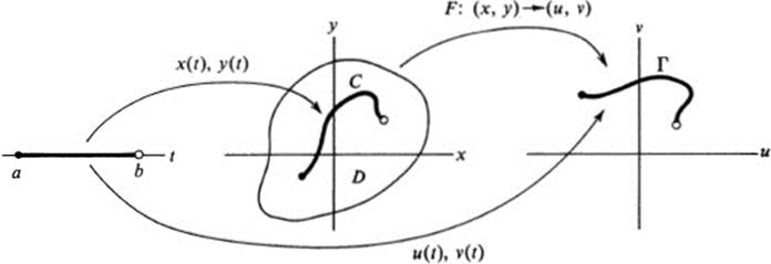
FIGURE 16.1Image of a curve under a mapping
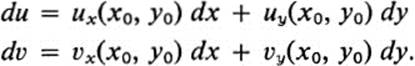
If F is a differentiable transformation, then the chain rule yields
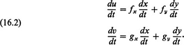
More precisely, if x0 = x(t0); y0 = y(t0), then
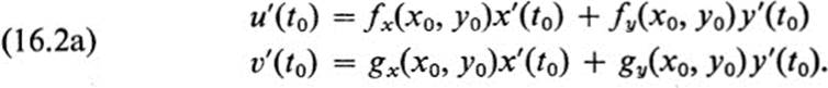
We use these equations to study the transformation F near an arbitrary point (x0, y0) in D. Let (u0, υ0) be the image of (x0, y0) under F, and let C be any curve passing through (x0,y0), where x0 = x(t0), y0 = y(t0). Note first that the coefficients fx, fy, gx, gy are all evaluated at the point (x0, y0), and do not depend on the choice of the curve C through the point. Furthermore, the right-hand side of Eqs. (16.2a) depends only on the tangent vector ![]() x'(t0), y'(t0)
x'(t0), y'(t0)![]() . As for the left-hand side, it defines precisely the tangent vector
. As for the left-hand side, it defines precisely the tangent vector ![]() u'(t0), υ'(t0)
u'(t0), υ'(t0)![]() to the image curve Γ. Our first conclusion is therefore the following.
to the image curve Γ. Our first conclusion is therefore the following.
Lemma 16.1Let F be a differentiable transformation near (x0, y0). Then all curves through (x0, y0) having the same tangent vector at (x0, y0) map onto curves having the same tangent vector at the image of (x0, y0).
This lemma is often expressed in the form: a differentiable transformation defines at each point an induced transformation of tangent vectors.
In order to see more clearly the nature of this induced transformation, let us introduce the notation:
![]()
Then Eq. (16.2a) takes the form of a linear transformation
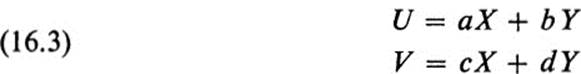
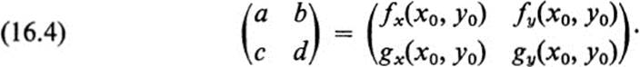
with matrix
We have therefore the further result.
Lemma 16.2Under a differentiable transformation F, the induced correspondence of tangent vectors at each point is a linear transformation.
Definition 16.2 The linear transformation (16.3) with matrix (16.4), associated with the transformation F at the point (x0, y0) is called the differential of F and denoted by dF.
RemarkIn using the notation dF it is always understood that a particular point has been chosen. If we wish to indicate the choice of this point we use the notation dF![]() Thus
Thus
![]()
is the linear transformation defined by (16.3) and (16.4).
Definition 16.3The transformation F is called singular at (x0, y0) if dF(x0, y0) is a singular linear transformation, and regular at (x0, y0) if dF(x0, y0) is nonsingular.
We recall that a linear transformation is singular if its determinant vanishes.
Definition 16.4 The matrix (16.4) is called the Jacobian matrix at (x0, y0) of the transformation F. We denote the Jacobian matrix by
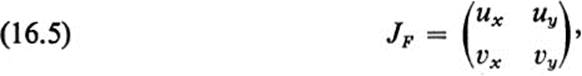
where u and υ are given as functions of x and y by (16.1), and it is understood that this matrix is associated with F at a given point.
Definition 16.5 The Jacobian of F at a point is the determinant of the Jacobian matrix at that point.
The standard notation for the Jacobian is

We note that the Jacobian of F is defined at each point of the domain D and is therefore itself a function in D.
Theorem 16.1Let F be a differentiable transformation in D, and let F map a point (x0, y0) of D into (u0, υ0).
Case 1.F is singular at (x0, y0).Then all differentiable curves C through (x0, y0) map into curves through (u0, υ0) whose tangent vectors lie along a single line.
Case 2.F is regular at (x0, y0). Then there is a one-to-one correspondence between tangent vectors to curves at (x0, y0) and tangent vectors to curves at (u0, υ0).
PROOF.In case 1, dF(x0, y0) is singular and maps all vectors (X, Y) into some line. We include in this case the possibility that all four partial derivatives ux, uy, υx, υy vanish at (x0, y0), in which case each curve C through (x0, y0) maps onto a curve whose tangent vector ![]() u'(t0), υ'(t0)
u'(t0), υ'(t0)![]() is zero.
is zero.
In case 2, dF(x0, y0) is nonsingular, and hence defines a one-to-one correspondence between ![]() X, Y
X, Y![]() and
and ![]() U, V
U, V![]()
![]() .
.
Example 16.1
Let F be the mapping u = x2, υ = y. Then
![]()
Hence
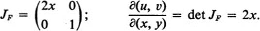
Thus F is regular at all points except along the y axis; on the y axis, where x = 0, F is singular.
Case 1.Let us look at a singular point, say (0, 1). Then F:(0, 1) → (0, 1). We wish to look at curves in the x, y plane through (0, 1) and their images under F. Since the tangent vector of the image; depends only on the tangent vector to the original curve, we get a complete picture by considering all straight lines through (0, 1). Thus, let C be the line
![]()
for any fixed α. The image Γ is given by
![]()
The point (0, 1) corresponds to t = 0. The tangent vector to C is
![]()
The tangent vector to Γ is
![]()
Hence the differential dF(0, 1) is the map
![]()
This means that the tangent vector to the image curve is always vertical. We can verify this explicitly by writing the curve Γ in nonparametric form. We have υ − 1 = t sin α, and
![]()
But this is just a parabola with vertex at (0, 1) (Fig. 16.2). Thus all straight lines through (0, 1) map onto parabolas with vertical tangent at (0, 1).
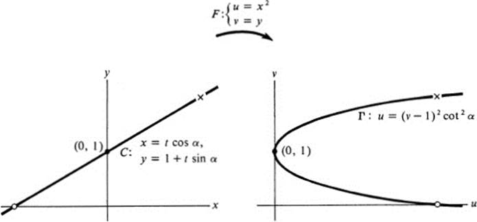
FIGURE 16.2 Map: F(x, y) → (x2, y) near a singular point
Case 2.Let us examine a regular point, say (1, 0). Again we may restrict our attention to straight lines through (1, 0). Every such line has the equation
![]()
The image is
![]()
This is again a parabola
![]()
The derivative is
![]()
At the point (1, 0) we have du/dυ = 2 cot α, and hence the slope is dυ/du = ![]() tan α. As α varies, we obtain as the image of lines through (1, 0) in the x, y plane, a family of parabolas through (1, 0) in the u, υ plane. The correspondence between tangents is one-to-one (Fig. 16.3).
tan α. As α varies, we obtain as the image of lines through (1, 0) in the x, y plane, a family of parabolas through (1, 0) in the u, υ plane. The correspondence between tangents is one-to-one (Fig. 16.3).
Definition 16.6 A transformation is called orientation-preserving at a point if its Jacobian is positive and orientation-reversing if its Jacobian is negative.
Recalling that the Jacobian of the transformation F is equal to the determinant of the linear transformation dF, we see from our discussion of the sign of the determinant in Sect. 14 that if we rotate a curve about a point (x0, y0) in the positive direction, then the image curve rotates in the same direction or the opposite direction, depending on whether the transformation F preserves or reverses orientation.
FIGURE 16.3 Map: F(x, y) → (x2, y) near a singular point
In Example 16.1, the Jacobian was equal to 2x, hence positive for x > 0 and negative for x < 0. Thus the transformation u = x2, υ = y is orientation- preserving in the right half-plane, and orientation-reversing in the left halfplane. If we recall that this transformation may be described roughly as “folding over the left half-plane onto the right” then the intuitive content of reversing orientation becomes quite evident.
We turn next to a somewhat different way of viewing the differential dF of a transformation. Applying the fundamental lemma of Chapter 2 (Lemma 5.1) to each of the functions u(x, y), υ(x, y), we may write

where F(x0, y0) = (u0, υ0), F(x, y) = (u, υ) and

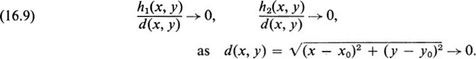
The remainder terms h1(x, y), h2(x, y) satisfy
If we temporarily ignore the remainder terms in Eq. (16.7), then the right-hand side is simply a linear transformation, namely dF![]() , applied to the displacement vector
, applied to the displacement vector ![]() x − x0, y − y0
x − x0, y − y0![]() rather than to the tangent vector
rather than to the tangent vector ![]() x'(t0),y'(t0)
x'(t0),y'(t0)![]() , and the left-hand side defines the corresponding displacement vector
, and the left-hand side defines the corresponding displacement vector ![]() u − u0, υ − υ0
u − u0, υ − υ0![]() We may therefore describe the content of the Eqs. (16.7) as follows.
We may therefore describe the content of the Eqs. (16.7) as follows.
Theorem 16.2 The differential dF![]() applied to the displacement vector
applied to the displacement vector ![]() x − x0, y −y0
x − x0, y −y0![]() yields the displacement vector
yields the displacement vector ![]() u − u0, υ − υ0
u − u0, υ − υ0![]() up to remainder terms satisfying (16.9) (see Fig. 16.4).
up to remainder terms satisfying (16.9) (see Fig. 16.4).
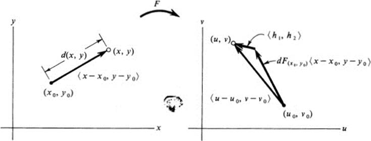
FIGURE 16.4 The differential dF(x0, y0)
In other words, every differentiable transformation F may be approximated near each point by a linear transformation, just as a differentiable function may be approximated by a linear function (namely, the tangent line to the graph of the function). It is for this reason that linear transformations play such a fundamental role in the study of arbitrary differentiable transformations.
Example 16.2
Let F be the transformation
![]()
Then
If we wish to study F near the point (1, 1), then we note that at that point
![]()
Equations (16.7) take the form
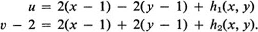
Thus the displacement vector ![]() u, υ − 2
u, υ − 2![]() is obtained from
is obtained from ![]() x, −1, y − 1
x, −1, y − 1![]() , up to remainder terms, by a linear transformation with matrix
, up to remainder terms, by a linear transformation with matrix
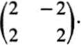
But we have seen in Sect. 15 that such a matrix defines a similarity transformation. In fact, if we divide each entry by 2![]() , we are left with the matrix
, we are left with the matrix
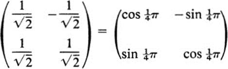
corresponding to a rotation of 45°. The approximate behavior of the transformation F near the point (1, 1) can then be described as follows (Fig. 16.5): take a neighborhood of (1, 1) and move it by a translation so that the point (1, 1) goes into (0, 2); then make a dilation about the point (0, 2) with a factor of 2![]() ; then make a rotation about (0, 2) through 45° in the positive direction. We note once again, that the linear transformation dF(x0, y0), which when applied in this way to displacement vectors at (x0,y0) gives the approximate behavior of F near (x0,y0), is the same one, which when applied to tangent vectors at (x0, y0), gives the precise tangent vector of the image. Thus Fig. 16.5is an exact description of the behavior of tangent vectors to curves through (1, 1) under the transformation F.
; then make a rotation about (0, 2) through 45° in the positive direction. We note once again, that the linear transformation dF(x0, y0), which when applied in this way to displacement vectors at (x0,y0) gives the approximate behavior of F near (x0,y0), is the same one, which when applied to tangent vectors at (x0, y0), gives the precise tangent vector of the image. Thus Fig. 16.5is an exact description of the behavior of tangent vectors to curves through (1, 1) under the transformation F.
In conclusion, we make the following observation. When trying to visualize an arbitrary differentiable transformation F near a point (x0, y0), it is often helpful to recall that the linear map dF(x0, y0) takes circles into ellipses, and since this map approximates F near (x0, y0), we should picture a small circle about (x0, y0) being mapped by F onto a curve that is approximately an ellipse. Furthermore, as we noted in Sect. 14, under the map dF the ratio of the area inside the image ellipse to the area inside the circle about (x0, y0) is equal to the absolute value of the determinant of dF, which is the Jacobian of F at (x0, y0). We saw earlier that the sign of the Jacobian had the geometric significance of distinguishing between orientation-preserving and -reversing transformations. We now have the important geometric interpretation of the magnitude of the Jacobian: the absolute value of the Jacobian of F at (x0, y0)is approximately equal to the ratio of areas of a small circle about (x0, y0) and its image under F. It should be remarked that this approximate statement can be replaced by an exact one, using a limiting procedure. We shall do so in Sect. 27. As an aid to our intuition, we anticipate to the extent of stating the following result (see Corollary to Th. 27.2): the Jacobian of F at (x0, y0) is precisely equal to the limiting value of the ratio of areas, where we choose a sequence of circles about (x0, y0) whose radii tend to zero.
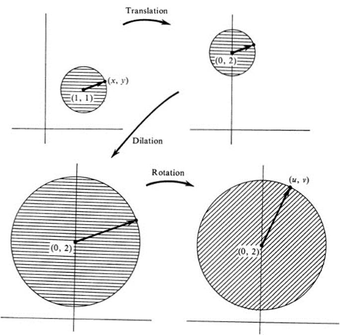
FIGURE 16.5 dF(1, 1)![]() x − 1 ,y−1
x − 1 ,y−1![]() ; where F: (x, y)→ (x2 − y2, 2xy)
; where F: (x, y)→ (x2 − y2, 2xy)
Exercises
16.1 Find the Jacobian matrix of each of the following transformations.
a. ![]()
b. ![]()
c. ![]()
d. ![]()
e. ![]()
f. ![]()
g. ![]()
h. ![]()
i. ![]()
j. ![]()
*k. 
16.2 For each transformation in Ex. 16.1, compute the Jacobian and determine the set of points in the x, y plane where the transformation is singular.
16.3Show that the Jacobian of a linear transformation F is constant, and coincides with the determinant of F.
16.4Let F be a differentiable transformation whose Jacobian is constant. Does F have to be linear? What if u and υ are known to be polynomials in x and y?
16.5Let F1 and F2 be differentiable transformations having the same Jacobian matrix at every point of a domain D. Show that F2 is the composition of F1 with a translation.
16.6Let F be an affine transformation
a. Find the differential dF at an arbitrary point (x0, y0).
b. What does your answer to part a imply about the remainder terms in Eq. (16.7) in the case of an affine transformation?
16.7 a. In Example 16.1, find dF(0, 1) by direct evaluation of the Jacobian matrix JF at the point (0, 1), and verify that the result is the same as that obtained in the text by examination of tangent vectors and their images.
b. In the same example, evaluate JF at the point (1, 0) and describe the corresponding linear transformation geometrically. Use this description to deduce the action of dF(1, 0) on tangent vectors as described in the text.
16.8At which points is the transformation u = x2, υ = y2 orientation- preserving, and at which points is it orientation-reversing? Try to picture this geometrically.
16.9Find the differential of the transformation F:u = x3 −3xy2, υ = 3x2y − y3 at the point (1, ![]() ), and use it to describe the behavior of F near that point, as in Example 16.2.
), and use it to describe the behavior of F near that point, as in Example 16.2.
16.10Show that for the transformation F:u = ex cos y, υ = ex sin y, the differential dF at an arbitrary point is a similarity transformation.
*16.11In Example 16.1 we showed that every line through the point (0, 1) mapped onto a parabola with vertical tangent at (0, 1). However, we assumed implicitly that the line was not horizontal; that is, α ≠ 0. Examine carefully the case of a horizontal line. Find its image, and find the tangent vector to the image at the point (0, 1). Explain away any apparent contradictions.
16.12 Let F be a differential transformation of the form u = f(x), υ = g(y).
a. What is the Jacobian matrix of F?
b. What is the Jacobian of F?
c. Under what conditions is F orientation-preserving at (x0,y0), and when is it orientation-reversing?
d. Give a geometric explanation of the answer to part c.
e. Give an intuitive explanation of why you would expect the absolute value of the Jacobian in this case to represent the “area magnification” at the point.
16.13Let F be a differentiable transformation : u = f(x, y), υ = g(x, y). Let C1 be the curve x = t, y = y0 (that is, the horizontal line y = y0 in parametric form), and let C2 be the curve x = x0,y = t. Let Γ1, Γ2 be the images of C1, C2under F. Let (u0, υ0) = F(x0,y0).
a.Show that the Jacobian matrix JF at (x0, y0) has the following geometric interpretation. If the columns of JF are considered as the components of vectors; namely
then T1 and T2 are tangent vectors at (u0, υ0) to the curves Γ1 and Γ2, respectively.
b. Indicate the situation described in part a by a sketch.
c. Show that T1 and T2 are the images under dF(x0, y0) of ![]() 1, 0
1, 0![]() and
and ![]() 0, 1
0, 1![]() , respectively.
, respectively.
d. Let x = x0 +λt, y = y0 + μt be the equations of an arbitrary straight ine C through (x0, y0), and let Γ be the image of C under F. Show that the tangent vector to C at (x0, y0) is λ![]() 1, 0
1, 0![]() + μ
+ μ![]() 0, 1
0, 1![]() , and that the tangent vector to Γ at (u0, υ0) is λT1 +μT2.
, and that the tangent vector to Γ at (u0, υ0) is λT1 +μT2.
e. Show that |∂(u, υ)/∂(x, y)|(x0, y0) is equal to the area of the parallelogramspanned by T1 and T2.
*16.14 Let F be defined by
Find ∂(u, υ)/∂(x, y) at the points
a. (1, 1)
b. (1, 2)
c. (2, 1)
16.15Let F be the transformation
Show that every circle about the origin maps into an ellipse (which may degenerate into a line segment or a point).
(Hint: use Exs. 10.29a and 14.25a.)
16.16Let a differentiable transformation F map a regular curve C onto a curve Γ. Show that if F is regular at every point of C, then Γ is a regular curve.
RemarkThe definition we have given for the differential of a transformation is one that has evolved gradually out of the formal differential notation that was used throughout the nineteenth century and is still presented in many elementary texts. In that notation the differential at the point (x0, y0) of a transformation F: (x, y) → (u, υ) is given by
In some presentations the “dx” and “dy” are interpreted as independent variables, in which case the right-hand sides of these equations simply define the linear equations that represent dF![]() In other treatments, these equations are considered as purely formal expressions that may be operated on in certain specified ways. (For example, dividing through by dt and interpreting the quotients du/dt, dx/dt, etc., as derivatives, we arrive at meaningful and correct equations; namely, the chain rule.) In either case, the choice of notation is such that the expressions dx and dy tend to take on a life of their own. This is especially true when these same expressions appear later on under integral signs. (See, for example, Sect. 21 on line integrals.) As a consequence, many students come away from a calculus course with the sensation that there is something mystical about differentials. We have tried to avoid this by dispensing with the dx, dy notation altogether. In fact, we did not mention differentials at all until discussing transformations, although we could have easily given a similar treatment of the differential of a function f(x, y). Namely, df(x0, y0) would be the linear function whose coefficients are fx(x0, y0) and fy(x0, y0). But it is precisely this function which enters into the definition of the tangent plane, and nothing is gained by the introduction of new terminology.
In other treatments, these equations are considered as purely formal expressions that may be operated on in certain specified ways. (For example, dividing through by dt and interpreting the quotients du/dt, dx/dt, etc., as derivatives, we arrive at meaningful and correct equations; namely, the chain rule.) In either case, the choice of notation is such that the expressions dx and dy tend to take on a life of their own. This is especially true when these same expressions appear later on under integral signs. (See, for example, Sect. 21 on line integrals.) As a consequence, many students come away from a calculus course with the sensation that there is something mystical about differentials. We have tried to avoid this by dispensing with the dx, dy notation altogether. In fact, we did not mention differentials at all until discussing transformations, although we could have easily given a similar treatment of the differential of a function f(x, y). Namely, df(x0, y0) would be the linear function whose coefficients are fx(x0, y0) and fy(x0, y0). But it is precisely this function which enters into the definition of the tangent plane, and nothing is gained by the introduction of new terminology.
There are, on the other hand, several advantages worth mentioning to the classical notation. First of all, it is sometimes easier to manipulate in computations. Secondly, the suggestive nature of the notation may lead one to certain formulas that can then be proved rigorously. Finally, by thinking of differentials as “small quantities,” applied mathematicians are often able to derive mathematical models for the objects of their study.
The student who wishes to familiarize himself with the manipulation of differentials in the classical notation should verify the formulas in Ex. 16.17.
16.17Let u = f(x, y), υ = g(x, y), w = φ(u, υ). Fix a point (x0, y0) at which differentials are evaluated. Using the notation
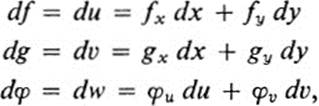
show that the following statements are valid.
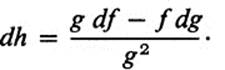
a. If h(x, y) = f(x, y)g(x, y), then dh = f dg + g df.
b. If h(x, y) = f(x, y)/g(x, y) and g(x0, y0) ≠ 0, then
c. If f(x, y)2 − g(x, y)3 ≡1, then 2f df = 3 g dg.
d. wu du + wv dυ = wx dx + wy dy.
(Hint: use, if necessary, Eq. (17.2a).)
e. If we introduce the notation r = ![]() x, y
x, y![]() , dr =
, dr = ![]() dx, dy
dx, dy![]() , then
, then
![]()