Two-Dimensional Calculus (2011)

Chapter 3. Transformations

19. Vector fields

At the beginning of this chapter we noted that one way in which pairs of functions arise is as the components of a vector field. We now investigate some of the basic concepts and problems that occur in this connection.

Definition 19.1 If u(x, y)∈ and υ(x, y) ∈ in a domain D, then the mapping that assigns to each point (x, y) in D the vector u(x, y), υ(x, y) is called a vector field in D.

A differentiable vector field is a vector field that is for some k ≥ 1.

We gave several examples in Sect. 13, including the vector fields obtained by forming the gradient of a given function.

Definition 19.2 A vector field u(x, y), υ(x, y) is called conservative, if there exists a function f(x, y) such that u(x, y), υ(x, y) = ∇f(x, y);the function f(x, y) is called a potential function for the field.

Remark Much of the terminology in the theory of vector fields is of physical origin. We do not try to explain each expression as it is introduced, but the physical interpretation will be discussed at an appropriate point.

By definition, if f(x, y) is a potential function, we have

In particular, for u, υ to be a differentiable vector field, the functions u = f_x and υ = f_y must be continuously differentiable, and hence f(x, y) must be in .

A natural question is the following: “how does one tell whether a given vector field is conservative; that is, equal to the gradient of some function?” The complete answer to this question turns out to have many fascinating ramifications, which we shall explore in the following chapter. There is, however, a partial answer that is easily given.

Lemma 19.1If a differentiable vector field u(x, y), υ(x, y) has a potential function in a domain D, then

throughout D.

PROOF. By assumption, there exists a function f(x, y) ∈ in D satisfying Eq. (19.1). By the equality of mixed derivatives (Th. 11.1) we have (f_x)_y = (f_y)_x which in view of Eq. (19.1) yields Eq. (19.2).

We should be clear as to the precise value of this lemma. It tells us that if a given vector field does not satisfy Eq. (19.2), then it cannot have a potential function. However, if Eq. (19.2) is satisfied, Lemma 19.1 does not allow us to assert that a potential function exists; furthermore if a potential function does exist, there remains the problem of how to find it. These are matters that we shall investigate in the next chapter.

There is one more elementary observation to be made here.

Lemma 19.2If a vector field in a domain D has a potential function, then this function is determined up to an additive constant.

PROOF. If f and g are potential functions of the same vector field, then they both have the same gradient, and by the Corollary to Th. 7.2, they differ by a constant.

Example 19.1

Let

To see if the vector field y, x is conservative, we check Eq. 19.2. We have u_y = 1, υ_x = 1. Hence, Eq. 19.2 holds, and a potential function may exist. If it does, we have f_x = y, f_y = x. But by inspection we can exhibit such a function: f(x, y) = xy.

Example 19.2

In this case u_y = −1, υ_x = 1. Equation (19.2) does not hold, and hence a potential function cannot exist.

Example 19.3

Here u, υ is a differentiable vector field in the domain D consisting of the whole plane except for the origin. We find that

Thus a potential function may exist. In this case it is not as easy as in Example 19.1 to construct a potential function explicitly. We shall return to this example in Sect. 22, where we shall show (in the discussion preceding Th. 22.2) that in fact there does not exist a potential function in D for this vector field.

It is a useful observation that when the vanishing of an expression, as for example in Eq. (19.2), is of fundamental importance, then a study of that expression itself is often fruitful. We shall in fact again meet the quantity

in connection with Green’s theorem (Sects. 25–27). At this point, we introduce a similar expression, which is also of importance.

Definition 19.3 If u(x, y), υ(x, y) is a differentiable vector field, then the quantity

is called the divergence of the vector field.

RemarkIt would be natural to consider expression (19.4) if for no other reason than that it represents the trace of the Jacobian matrix

of the pair of functions u(x, y), υ(x, y). We have seen that the trace of a matrix plays a basic role in the theory of quadratic forms, and in fact the trace and the determinant are the two most fundamental quantities associated with a given matrix.

We now introduce two important classes of vector fields.

Definition 19.4A differentiable vector field u(x, y), υ(x, y) in a domain D is called solenoidal or divergence-free if it satisfies

throughout D.

Definition 19.5 A differentiable vector field that satisfies both Eqs. (19.2) and (19.5) is called a harmonic vector field.

The reason for this terminology is the following.

Lemma 19.3If f(x, y) is the potential function of a differentiable vector field u(x, y), υ(x, y) , then u(x, y), υ(x, y) is a harmonic vector field if and only if f(x, y) is a harmonic function.

PROOF. Since u = f_x and υ = f_y, Eq. (19.2) automatically holds, and since u_x + υ_y = f_xx + f_yy, Eq. (19.5) is equivalent to f harmonic.

In case it may have passed unobserved, we call attention to the fact that the pair of Equations (19.2) and (19.5) are precisely the same as the Eqs. (18.4), which arose in connection with Conformal mapping. This is a striking example of what is often called the “unity of mathematics.” The investigation of two apparently totally unconnected subjects, such as a geometric question about angle-preserving transformations, and a class of vector fields that arise in physics, may lead to precisely the same mathematical formulation—in this case, the same pair of equations that must be satisfied.

We conclude this section with a brief description of some of the physical problems that led to the consideration of the above types of vector fields. Historically, in the theory of vector fields the physical interpretation and the mathematical treatment have gone hand in hand, each aiding in the development of the other. Most of the early theorems in the subject were inspired by physical considerations. The most famous example of the reverse development is Maxwell’s theory of electromagnetism, in which mathematical reasoning led Maxwell to predict the existence of electromagnetic waves, including the many familiar types since discovered—radio, radar, cosmic rays, etc. We should emphasize, however, that no knowledge of physics is required to understand the mathematical material presented in this book. To the extent that one or another physical interpretation aids the intuition, it should certainly be utilized; wherever it does not, it can be ignored.

Heat Flow

A simple example of a function of two variables is provided by the temperature at each point on the bottom of a frying pan, which is being heated by a gas burner. A somewhat idealized version of the same situation is the following. Suppose that constant heat sources are applied at different points along the circumference of a metal disk, and enough time is allowed to elapse so that the temperature distribution attains an equilibrium. The temperature then becomes a function of position, and the gradient of the temperature is a vector field which at each point indicates the direction and magnitude of heat flow. This vector field is therefore conservative. From the fact that there are no heat sources in the interior of the disk, it can be shown that the vector field is also divergence-free, and hence is a harmonic vector field. By Lemma 19.3, the temperature, which is the potential function of the field, is a harmonic function. Conversely, given a harmonic function in a disk, one may picture it as defining a temperature distribution, and its gradient defines the vector field of heat flow.

We may mention that this physical interpretation accounts very nicely for the property of harmonic functions known as the “maximum principle” (see Example 11.6). Namely, if a harmonic function, pictured as the potential function of a steady heat flow, had a local maximum at a point, then the heat would be flowing away from that point, and the temperature would not have reached an equilibrium.

Fluid Flow

Consider the flow of a liquid or gas enclosed in a tube. The tube may have variable diameter, and the velocity of flow may vary from point to point, but we assume that the velocity at each point does not vary with time. Let us further assume that the flow can be represented by a lateral section of the tube (Fig. 19.1). The parhysical situation may then be described by a velocity field; that is, a vector field such that the magnitude and direction of the vector at each point represents the speed and direction of flow at that point. We shall return frequently to this physical model of a vector field, and we shall see that various quantities, such as the divergence, are most easily visualized in terms of such a flow.

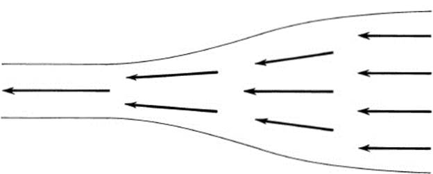
FIGURE 19.1 Velocity field of flow in a tube

Force Fields

Assume, as an approximation, that the sun, planets, and other bodies in the solar system lie in a plane. If a particle of unit mass is placed at some point in this plane, it is attracted to each of these objects in varying degree, and the total effect is that of a force exerted on the particle, imparting to it a given acceleration in a given direction. The magnitude and direction of this force determines a vector, and the set of all vectors obtained in this way (by placing the particle at arbitrary points) defines a vector field called a gravitational force field. Theoretically, the force field determines the path any particle follows if it is placed at an arbitrary point either at rest or with an arbitrary initial velocity. It is a consequence of Newton’s laws that the gravitational force field (at all points outside the solar bodies) is a harmonic vector field.

Similarly a distribution of electrostatic charges determines a force field, which in turn determines the motion of a charged particle placed in the field. Perhaps the simplest force field to visualize is a magnetic field, whose direction at each point is found by placing a magnetic compass at the point and observing the direction of the needle. The term “solenoidal” for a vector field originated in the properties of a magnetic field inside a solenoid.

For further discussion of these matters from the physical point of view, we refer to references [9], [33].

Exercises

19.1For each of the following vector fields u(x, y), υ(x, y) , compute the divergence, and decide which vector fields are solenoidal.

a. a, b , a and b constants

b. (ax, by) , a and b constants

c. φ(x), ψ(y) , φ(y) and ψ(y) continuously differentiable

d φ(y), ψ(x) , φ(y) and ψ(x) continuously differentiable

e. 2xy, x²

f. − x² + y², 2xy

g. 2yx², 3x²y

h. e^{x + y}, e^{x −y}

i. sin x cos y, cos x siny

j. y/x, log x

k. e^x cos y, e^x siny

I. e^x sin y, e^x cosy

19.2For each of the vector fields in Ex. 19.1, decide whether or not it is conservative, and if so, find a potential function.

19.3Which of the vector fields in Ex. 19.1 are harmonic vector fields?

19.4Which of the following vector fields are harmonic vector fields?

a. x + y, x − y

b. x² + y², 2xy

c. x³ − 3x² + 3x − 3xy² + 3y² − 1, y³ − 3yx² + 6yx − 3y

d. −y/(x² + y²), x/(x² + y²)

e. log (x² + y²), 2 arc tan y/x

19.5Show that if a vector field u, υ is conservative, then the vector field is solenoidal.

19.6Let w = u, υ be a harmonic vector field.

a. Show that u and υ are harmonic functions.

b. Show that for any constant vector d, the projection of w in the direction of d is a harmonic function.

19.7Given f(x, y) ∈ in a domain D, consider the vector field w = ∇f. Express the divergence of the vector field w in terms of f.

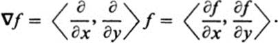
19.8 A revealing way to think of the gradient operator ∇ is as a “vector valued operator,” which assigns to each function f, the vector field ∇f. Symbolically, we may write

meaning

This leads us to write

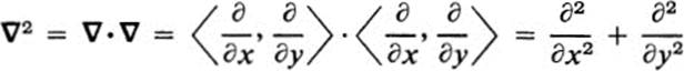
meaning

(The operator ∂²/∂x² + ∂²/∂y² is called the Laplacian, and is also frequently denoted by Δ. Thus, if f(x, y) ∈ , the Laplacian of fis Δf = ∇²f= f_xx + f_yy.) For a vector field w = u, υ we write

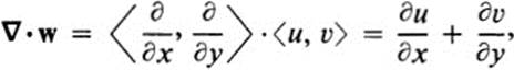
which is the divergence of w.

Show that the following equations involving this notation are valid.

a. ∇²f = ∇·(∇f)

b. ∇·(fw) = (∇f)·w + f(∇· w)

c. ∇ · (f(∇g − g∇f) = f∇²g - g∇²f

d. ∇²(fg) = f∇²g + g∇²f + 2(∇f·∇g)

19.9For each of the following functions f(x, y), find the vector field u, υ = ∇f. Try to visualize the vector field by sketching a number of its vectors, where the vector u(x, y), υ(x, y) is drawn as a displacement vector starting at the point (x, y). (See, for example, Fig. 13.3.)

a. f(x, y) = x

b. f(x, y) = 2x + y

c. f(x, y) = x² + y²

d. f(x, y) = x² + 2xy+ y²

e. f(x, y) =y/x

f. f(x, y) =

19.10If the plane is rotated about the origin with a constant angular velocity ω, then a point with coordinates (x₀, y₀) at time t = 0 has coordinates (x, y) at time t, where

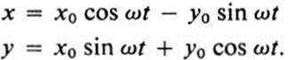
This motion defines a velocity field that may be described as follows: at any time t₁, the velocity vector at the point (x(t₁), y(t₁)) is given by u, υ = x'(t₁), y'(t₁) .

a. Show that this vector field does not depend on the time, but only on the position. In fact, x'(t₁), y'(t₁) = ω −y(t₁), x(t₁) so that u(x, y), υ(x, y) = ω(−y, x

b. Sketch this vector field, choosing the constant ω = .

Remark: given a vector field u(x, y), υ(x, y) in a domain D, a regular curve C is called an integral curve of this vector field if the tangent vector to C at each point has the same direction as the vector field at that point. If the curve is given by x(t), y(t), this means that if x₀ = x(t₀), y₀ = y(t₀), then x'(t₀), y'(t₀) should have the same direction as u(x₀, y₀), υ(x₀, y₀) . The problem is essentially that of solving a pair of simultaneous differential equations:

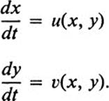
However, since it is only the direction of the vectors that must coincide, the problem is really that of solving the single equation

where F(x, y) = υ(x, y)/u(x, y), which is obtained by dividing the second equation above by the first. This problem is discussed in detail in books on differential equations (see, for example, [1]). As an aid in visualization, it is useful to picture the vector field as the velocity field of a fluid flow. Then if we follow the motion of a particle carried along by the flow, it describes a path whose direction at each point is the direction of the velocity field at that point. These paths are called stream lines of the flow, and we see that stream lines are precisely integral curves of the vector field. A function g(x, y) is called a stream function of the flow, if its level curves g(x, y) = c are stream lines. Examples and further comments are given in Exs. 19.11–19.15.

19.11Sketch each of the following vector fields. Show that the given function g(x, y) is a stream function, and sketch some of the stream lines.

a. 1, 0 ; g(x, y) = y

b. y, 0 ; g(x, y) = y

c. −y, x ; g(x, y) = x² + y²

d.

19.12Show that g(x, y) is a stream function of a vector field w = u, υ if and only if ∇g⊥ w at each point. Verify that this is the case for each part of Ex. 19.11.

19.13Let f(x, y), g(x, y) define a harmonic vector field. Show that g(x, y) is a stream function for the vector field ∇f, and f(x, y) is a stream function for the vector field ∇g.

19.14Let

a. Show that the vector field w = ∇f has the following properties:

(1) it is horizontal along the x axis

(2) it is tangent to the unit circle x² + y² = 1 at every point of that
circle

(3) it vanishes at the points (1,0) and (−1,0)

(4) it tends to the constant vector field 1, 0 as x² + y² → ∞.

b. Using the properties in part a, make a very rough sketch of the vector field w in the domain D consisting of the entire exterior of the unit circle. See if these properties coincide with what you might visualize to be the velocity field of the following flow: a fluid is flowing uniformly in the positive x direction, with velocity vector 1, 0 throughout the plane; then an obstacle in the form of a circular disk is placed at the origin and the fluid is constrained to flow about the obstacle.

c. Verify that f(x, y), g(x, y) is a harmonic vector field, and hence, by Ex. 19.13, g(x, y) is a stream function of the vector field in part a.

d. Sketch several level curves g(x, y) = c (or rather, the part of the level curves lying outside x² + y² = 1), including the case c = 0, and compare the form of these curves as stream lines with the properties of the flow described in part a. (Hint: write the curve in the form x² = h(y). Show that h(y) ≥ 0 in an interval, at one end of which x = 0, and at the other end x → ∞. Thus the curve lies in a horizontal strip and has a horizontal asymptote.)

*19.15Let F be a diffeomorphism of a domain D onto a domain E.

a. Show that the differential dF assigns in a natural way to each vector field v in D a vector field w in E.

b. Show that if v and w are as in part a, then F maps integral curves of v onto integral curves of w.

19.16The force field set up by a charged particle placed at the origin is given by

a. Show that this field is conservative and that − log (x² + y²) is a potential function.

b. Show that this field is solenoidal.