Two-Dimensional Calculus (2011)

Chapter 3. Transformations

20. Change of coordinates

Having discussed pairs of functions first from the point of view of plane mappings, and then as vector fields, we come now to our third and final interpretation, that of coordinate transformations. We begin with a few general remarks on coordinate systems.

We note first that a function is usually defined by assigning a number to each point of some set. Thus, we may assign to each position on a mountain range its altitude above sea level, or to each point on a frying pan its temperature at a given time. Only later, after each point of the set has been assigned coordinates, can the function be expressed in an explicit form, such as x², or x + cos y. If the function represents the curvature of a railroad track, then it can be represented as a function of one variable, since we can identify each point along the track by a single coordinate, such as the distance along the track from a fixed point. To represent temperature in the atmosphere would require a function of three variables, since each point is identified by three coordinates. The two-dimensionality of the plane, translated into our terms, means that each point can be represented by a pair of coordinate's. This may be done in many different ways; in order to study a particular function we may choose coordinates that are most convenient for that purpose. Thus, when we were presented with a quadratic form ax² + 2bxy + cy², we found it useful to make a rotation of coordinates,

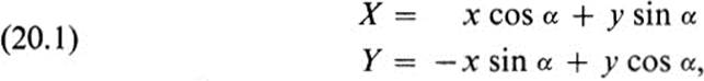
so that in the new coordinates the same function would be represented as AX² + CY².

If (x, y) are rectangular coordinates, then the new coordinates (x, y) given by Eqs. (20.1) are rectangular also, meaning that the “coordinate curves,” X = c, Y = d, are straight lines intersecting at right angles. It is often useful to consider more general systems of coordinates. All that is needed is a method of assigning a unique pair of numbers x, y to each point, as a means of quantitatively distinguishing one point from another. If we had previously chosen some other coordinate system, which assigned a pair of numbers x, y to each point, then X and Y would each be a function of the two variables x, y; that is,

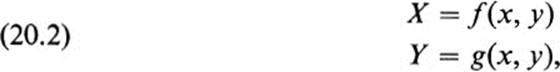
where f and g are specific functions. One sometimes uses the expression “curvilinear coordinates” for the general case in which the coordinate curves X = c, Y = d are not straight lines. The crucial property is that the curves X = c, Y = d should intersect at a unique point, so that this point may be identified in the new coordinate system by the pair of values (c, d) (Fig. 20.1).

Conversely, given any pair of functions f(x, y), g(x, y) such that Eqs.(20.2) set up a one-to-one correspondence between (x, y) and (x, y), we may use these equations to define new coordinates.

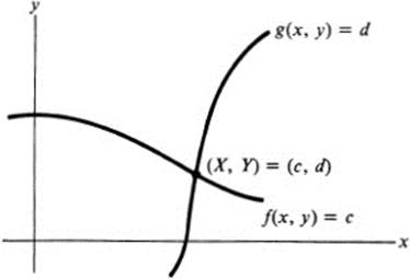
FIGURE 20.1Curvilinear coordinates

Example 20.1

Let (x, y) be Cartesian coordinates, and let

Here the coordinate curves X = c, Y = d, are circles about the origin and rays from the origin, respectively (Fig. 20.2). The coordinates X, Y are called polar coordinates, and are more commonly designated as r, θ.

There are two points that should be made in connection with general coordinate systems. The first is that a particular coordinate system may not be defined in the whole plane, but only in some domain D. For example, the functions f(x, y), g(x, y) used in Eq. (20.2) may be defined only in a part of the plane. Thus, in the case of polar coordinates, the function tan⁻¹ (y/x)

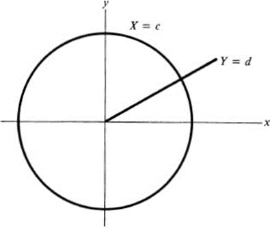
FIGURE 20.2Polar coordinates

is not defined at the origin, and it is not defined in a single-valued way in the rest of the plane. To avoid all difficulties we must restrict polar coordinates to some domain D (such as the first quadrant, or the upper half-plane) in which it is possible to select a single-valued branch of tan⁻¹ (y/x).

Secondly, in order to be able to apply calculus, the relation between coordinate systems should be sufficiently differentiable so that the derivatives of a function with respect to one coordinate system can be computed in terms of its derivatives with respect to the other.

Suppose then that u(x, y) is continuously differentiable, and let new coordinates X, Y be introduced by Eq. (20.2). Then u becomes a function of x, y, and using the chain rule, we have

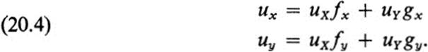
These equations may be solved to express u_X, u_Y in terms of u_x, u_y providing the determinant is not zero. But the determinant is f_xg_y − g_xf_y, the Jacobian of f and g with respect to x and y. Our basic requirements for change of coordinates—that there should be a one-to-one correspondence between the pairs x, y and X, Y, such that each pair is given by continuously differentiable functions of the other—are precisely the conditions stated in Th. 17.2, in the context of transformations, guaranteeing that the Jacobian cannot vanish at any point.

Example 20.2

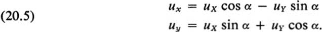
A rotation of coordinates, given by (20.1), is of the form (20.2) with

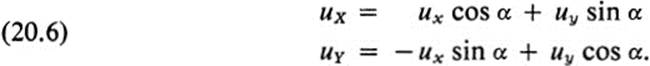
Substituting into (20.4), we have

Solving for u_X, u_Y, we obtain

Similarly, we can compute derivatives of arbitrary order. For example, applying the chain rule to the function u_X, we find

and similarly for u_Y. Thus, differentiating the first equation of (20.4) with respect to x, we have

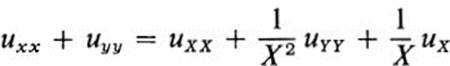
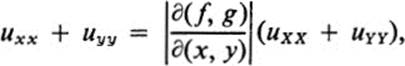
In a similar fashion we can express all partial derivatives of u with respect to x, y in terms of its derivatives with respect to X, Y and the derivatives of the change-of-coordinate functions f, g. We note here the expression for the Laplacian,

It is quite clear that if we are too capricious in our choice of new coordinates, then the expressions for most basic quantities become unmanageable. There are, however, many possible choices that greatly simplify these expressions (see, for example, Exs. 20.1, 2). If we substitute f(x, y) = (x² + y²)^1/2, g(x, y) = tan ⁻¹ (y/x) into (20.8), then we find the expression for the Laplacian in polar coordinates

or, in the more usual notation, with X = r, Y = θ,

Since (ru _r)_r = ru_rr + u_r = r(u_rr+ u_r/r), we may rewrite Eq. (20.9) in the form

Let us note just one consequence of this formula.

Lemma 20.1 If u(x, y) is a harmonic function that depends only on the distance r to the origin, then

for suitable constants c and d.

PROOF. If we express u in polar coordinates, then u_θ = 0, and since u is harmonic, Δ u = 0. From Eq. (20.10), we have

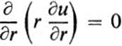
or

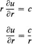
from which Eq. (20.11) follows immediately.

We consider next what happens to the components of a vector under a change of coordinates. We restrict ourselves to the case of a rotation of coordinates, given by Eqs. (20.1). We recall that the components with respect to a given coordinate system were originally defined in terms of a displacement vector as the difference in coordinates between the beginning and the endpoint. Thus, in the original coordinate system the components would be

while the new components would be

(Fig. 20.3). Substituting the coordinates of the beginning and endpoints in Eq. (20.1), and subtracting, we obtain

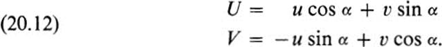
Using this fact about displacement vectors as a model, we use Eqs. (20.12) to define the new components U, V of an arbitrary vector, after the rotation of coordinates (20.1), if the vector had components u, υ with respect to the original coordinate system. Thus the relation (20.12) between the old and new components of a vector is precisely the same as that between the old and new coordinates of a point.

Let us consider, for example, a function f defined in the plane. It has one expression with respect to the coordinates x, y, and another with respect to

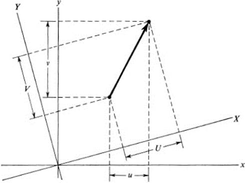
FIGURE 20.3 Components of a vector in different coordinate systems

X, Y. At each point we can consider the vector

which is the gradient of f with respect to the coordinates x, y. By Eq. (20.12), the components of this vector with respect to the new coordinates X, Y are given by

But using Eqs. (20.6), we find that Eq. (20.14) reduces to

This computation shows that the pairs of partial derivatives f_x,f_y and f_X, f_Y represent the components of the same vector with respect to two different coordinate systems. If we carry out an analogous computation with other pairs, such as f_x, −f_y and f_X, −f_Y, or f_y, f_x and f_Y, f_X, we find that these do not represent the same vector. Of course, this is not fortuitous, but is a consequence of the fact that the gradient of a function may be described in an intrinsic fashion in terms of the direction and magnitude of the maximal directional derivative. Since this characterization is independent of coordinates, it follows that whatever expression we obtain for the gradient vector in one (Cartesian) coordinate system must be valid in any other.

We examine next the case of an arbitrary differentiable vector field in some domain D. Again, we assume that we have two coordinate systems x, y and X, Y related by (20.1). Let the components of this vector field be u, v and (U, V with respect to the two systems, respectively. Each of the four quantities u, υ, U, V may be considered as functions of either x, y or X, Y. Differentiation of the first equation in (20.12) yields

Inserting the first of Eqs. (20.6) (and the analogous equation for the function υ), we obtain

In a similar way, we may express the other partial derivatives U_Y, V_X, and V_Y in terms of u_x, u_y , υ_x, υ_y. We note the result for V_y:

Adding (20.16) and (20.17), we find

Equation (20.18) states that the divergence of a vector field assigns to each point a number in an “invariant” manner; that is, independent of the choice of (Cartesian) coordinates. As in the case of the gradient, it is the particular combination of derivatives that has this property, and had we considered other expressions, such as u_x − υ_y, or u_y + υ_x, the analog of (20.18) would not hold. Unlike the gradient, the divergence has not been described up to now in any intrinsic fashion. However, its invariance under coordinate change, proved above by a purely formal computation, leads us to suspect that there should be a coordinate-free description, from which Eq. (20.18) would follow immediately. We shall, in fact, be able to give just such a description of the divergence of a vector field in Sect. 27, but only after we have developed the basic properties of integration in several variables.

Exercises

20.1For each of the following change-of-coordinate functions X = f(x, y), Y = g(x, y), use Eq. (20.8) to express u_xx + u_yy in terms of the new coordinates X, Y.

a.

b.

c.

20.2Show that if f(x, y), g(x, y) define a Conformal mapping and if we introduce new coordinates X = f(x, y), Y = g(x, y), then

so that a function u is harmonic with respect to x, y if and only if it is harmonic with respect to X, Y.

20.3Show that if the coordinates (X, Y) are obtained from (x, y) by a rotation of axes, then u_xx + u_yy = u_XX + u_YY.

20.4Carry out the derivation of Eq. (20.9) from Eq. (20.8).

20.5Show that for any integer n the function u(x, y) that takes the form rⁿ cos nθ in polar coordinates is a harmonic function.

20.6 a. Write down the form that Eqs. (20.4) take when X and Y are polar coordinates r, θ, and compute

b. Solve the equations in part a for u_r, u_θ in terms of u_x, u_y.

c. Let u(x, y) and υ(x, y) satisfy the Cauchy-Riemann equations. Find corresponding equations, which relate the partial derivatives of u and υ with respect to r and θ.

d. Show that the functions u(x, y), υ(x, y) which are given in polar coordinates by rⁿ cos nθ, rⁿ sin nθ, satisfy the Cauchy-Riemann equations.

e. Let n be a positive integer. Study the transformation F: u(x, y), υ(x, y) which takes the form R = rⁿ, φ = nθ, if polar coordinates (r, Θ) and (R, φ) are introduced in the x, y plane and u, υ plane, respectively. Describe this transformation geometrically, and show that it is a diffeomorphism of the angular sector 0 < θ < π/n onto the upper half-plane. Using part d, show that it is a Conformal mapping.

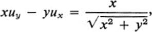
20.7Let u(x, y) ∈ in the upper half-plane and xu_y ≡ yu_x. Show that there exists a function g(t) of one variable such that u(x, y) = g(x² + y²). (Hint: see Exs. 7.26 and 7.27, and use Ex. 20.6a.)

20.8Find the function u(x, y) defined for all (x, y) ≠ (0, 0), which satisfies the equation

with u(x, 0) = 0 for all x ≠ 0. (Hint : see Ex. 20.7.)

20.9Find the most general form of a harmonic function in the upper halfplane that is constant along each ray through the origin.

20.10Show that if u(x, y) ∈ in the whole plane, and u_xy ≠ 0, then there exist functions G(t), H(t) of one variable such that u(x, y) = G(x) + H(y). (Hint: use Ex. 7.26 to show that u_x = g(x), u_y = h(y). Set

and use the Corollary to Th. 7.2.)

20.11The equation

where c is a nonzero constant, is called the one-dimensional wave equation.

a. Show that under the change of variables X = x − ct, Y = x + ct, we have

b. Show that if u(x, t) ∈ in the whole plane and u(x, t) satisfies the wave equation, then u(x, t) is of the form

(Hint : use part a and Ex. 20.10.)

20.12Derive the expressions for u_xy and u_yy analogous to Eq. (20.7) for u_xx.

20.13 a. Show that under the change of coordinates x = e^x, y = e^Y, we have

b. Use part a to write down some solutions of the equation

and then verify directly that this equation is satisfied.

20.14 a. Let a, b, c be arbitrary constants. Show that under a rotation of coordinates defined by Eqs. (20.1), we have

and find the explicit expressions for A, B, C in terms of a, b, c and α (Hint : use the expressions in Ex. 20.12.)

b. Show that as a special case of part a,

(In particular, the expression u_xx − u_yy is not invariant under a rotation of coordinates, as is u_xx + u_yy by Ex. 20.3.)

c. Let q(x,y) = ax² + 2bxy + cy². Show that under the rotation of coordinates defined by (20.1),

where A, B, C are given by the same expressions as in part a.

d. Let λ_l, λ₂ be the maximum and minimum of the quadratic form q(x, y) of part c subject to the condition x² + y² = 1. Show that under a suitable rotation of coordinates,

*20.15Find the most general function u(x, y) that satisfies the equation 3 u_xx + 10u_xy + 3u_yy = 0, throughout the plane. (Hint: use Exs. 20.14d and 20.11b.)

20.16 a. Show that under the change of coordinates X = kx, Y = ly, we have

thus, choosing k = and l = , both coefficients can be reduced to ± 1.

b. Show that under a suitable linear change of coordinates in each case, every sum of second-order derivatives with constant coefficients can be reduced to one of the following three forms:

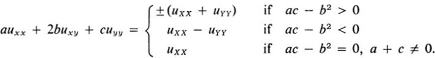
(Hint: use the composition of two linear transformations, first applying Ex. 20.14d, and then Ex. 20.16a.)

c. Find the most general function u(x, y) that satisfies u_xx ≡ 0 throughout the plane. Deduce that all solutions of the equation au_xx + 2bu_xy + cu_yy = 0 in the whole plane can be written down explicitly in case ac − b² < 0 or ac — b² = 0, whereas for ac − b² > 0 they can be expressed in terms of solutions to Laplace’s equation Δu = 0.

*20.17 a.Let X = f(x, y), Y = g(x, y) define a change of coordinates. Let . (x₀, y₀) be a point such that either

(1) u_x(x₀, y₀) = 0 and u_y(x₀, y₀) = 0, or

(2) the second derivatives of f and g are all zero.

Show that at the point (x₀, y₀), the expressions derived in Ex. 20.12, together with Eq. (20.7), can be summarized in a single matrix equation:

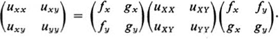
(Note: matrix multiplication is discussed in the Remark following Ex. 15.21.)

b. Show that under the hypotheses of part a,

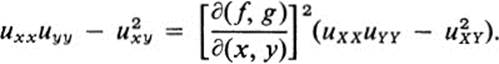
c. Show that under the hypotheses of part a,

where

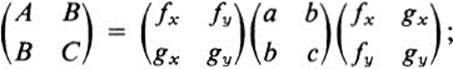
show that this equation contains as a special case the answer to Ex. 20.14a.

d. Let the functions f(x, y), g(x, y) of part a define a dififeomorphism F. For any numbers r, s, let

Show that under the hypotheses of part a,

where the derivatives on the left are evaluated at the point (x₀, y₀) and those on the right are evaluated at the corresponding point (X₀, Y₀) = (f(x₀, y₀), g(x₀, y₀)).

e. Show that under the hypotheses of part a, the quadratic form for the second directional derivatives has the same nature whether computed with respect to x, y or X, Y; in other words,

and

are simultaneously positive definite or negative definite, or positive semidefinite, etc.

f. Let F be the diffeomorphism X = f(x, y), Y = g(x,y); given a surface z = h(x, y), consider the corresponding surface z = (x, y), where = h F (see Ex. 17.4). Give a geometric interpretation of part e in terms of these two surfaces. (Note that if F is linear, then hypothesis 2 of part a holds at every point, and therefore so do all sùbsequent parts of this exercise, for an arbitrary function u(x, y). On the other hand, for an arbitrary diffeomorphism F, these results are valid at any point where ∇u = 0.)

20.18Verify Eq. (20.17) and derive similar expressions for U_Y and V_x.

20.19Using Eqs. (20.16) and (20.17) and the answer to Ex. 20.18, transform each of the following expressions into expressions involving u_x, u_y, υ_x, υ_y.

a. U_X − V_Y

b. U_X + V_Y

c. U_Y − V_X

20.20Show that if u, υ is a harmonic vector field, then the corresponding vector field U, V obtained by rotating coordinates is also harmonic.

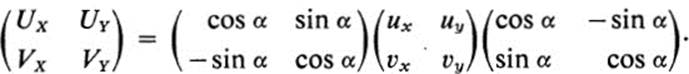
*20.21 a. Show that Eqs. (20.16) and (20.17) and the answer to Ex. 20.18 can be written in the form of a single matrix equation.

b. Show that U_XV_Y − U_YV_X = u_xυ_y − u_yυ_x.

RemarkIt may have become apparent in the course of these exercises that the standard notation that we have been using may lead to some real difficulties. These become even more serious later on, when dealing with functions of more than two variables. To cite one example, if w is given as a function of the three variables x, y, z, and if z is in turn a function of x and y, then what is meant by ∂w/∂x? It can have two interpretations, depending on whether we hold y and z fixed and let x vary, or we substitute z as a function of x and y and consider w just as a function of x and y. In the latter case, for fixed y, as x varies z also varies. Thus the notation ∂w/∂x should not be used in that situation, but be replaced by a more precise notation. Also in the present section, any possible confusion concerning the notation u_x and u_x could be avoided by writing u = h(x, y) and u = (x, y), where (x, y) = h(f(x, y), g(x, y)). Then h_x, h_Y should be related to _x, _y.

It may be appropriate in this connection to touch on a basic problem in functional notation. Consider, for example, the question “what happens to the function f(x, y) under a rotation of coordinates?” This question, taken at face value, is meaningless. The function f(x, y) assigns to every pair of numbers a third number. If f(x, y) = x² + y, then f(π, 1) = π² + 1, f(X, Y) = X² + Y, f(r, θ) = r² + θ. What is implied in the above question is that we consider the pair of numbers x, y to define a point p in the plane; we use the function of two variables f(x, y) to define a function, say g, which assigns to each point p of the plane a number g(p) by the rule g(p) = f(x, y) if (x, y) are the coordinates of the point p in the given coordinate system. Then if the point p is represented by (X, Y) in terms of a new coordinate system, we may define a new function of two variables, say (X, Y), by setting (X, Y) = g(p). The question then, is how this new function (X, Y) is related to the original function f(x, y).

The problem, in brief, is whether in speaking of a function f, we mean a point function (such as g(p) in the above discussion), which assigns a number to each point, and which takes on different forms in different coordinate systems, or a function of two variables, which assigns a fixed number to each pair of numbers according to a given rule, and which has nothing to do with the choice of coordinates. The fact is that both meanings are in common use, and in any given case the intended meaning must be deduced from the context. The important thing is to understand precisely what is meant in a given situation, and then the notation should not pose any problems. In some cases a more cumbersome notation is desirable in order to eliminate any possible confusion, but in others it may defeat one of the basic purposes of mathematical symbolism, which is to compress a large amount of information into compact form. It is well to remember that mathematical notation can be an invaluable aid to thought, but it cannot be a substitute for thought.

¹ See, for example, Section 12.4 of [36]. A proof which is purely two-dimensional is given in Ex. 26.29 of this book. Other proofs may be found in Chapter III, Section 3 of [11], and in Section 8.4 of [19].

² The term “Conformal mapping” is sometimes used to include more general mappings whose Jacobian is different from zero and which preserve angles, even if the mappings are not one-to-one in the whole domain. An example is the mapping u = x² − y², υ = 2xy, where the domain D is the whole plane minus the origin. Note that Th. 18.2 is valid for such mappings.

³ See also Fig. 16.5 and the related discussion of the behavior of this transformation near the point (1, 1).