Two-Dimensional Calculus (2011)
Chapter 4. Integration
23. Area
The object of this and the following section is to develop the notion of double integration. Rather than present the theory in detail, we prefer to stress certain points and merely sketch others. There are two reasons for this mode of presentation. The first is that the theory of multiple integration is essentially identical for any number of variables, and one may as well present it in general form at the appropriate place. The second is that there is a large gap between theory and practice in multiple integration. In practice, multiple integrals are almost invariably reduced to a succession of ordinary integrals. Thus, for our present purposes, as well as for most elementary applications, the principal properties of double integrals are those stated in Th. 24.3, and in Th. 24.4 and its Corollary. Our aim, therefore, is to present first some of the fundamental ideas and then to proceed to the properties needed in applications.3
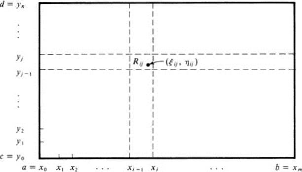
FIGURE 23.1 Subdivision of a rectangle for defining the double integral
To begin, consider a function f(x, y) defined on a rectangle
![]()
To define the double integral of f over R, we proceed exactly as in the case of the single integral. Divide the rectangle R into a number of smaller rectangles
![]()
where
![]()
(see Fig. 23.1). Choose an arbitrary point (ξij,ηij) in the rectangle Rij and
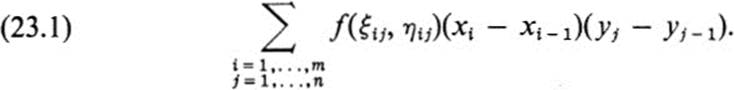
form the sum
If these sums tend to a limit as the size of the subdivisions tends to zero, then f(x, y) is said to be integrable, and the value of the limit is called the double integral of f over R. Analogs of the basic properties of integration in one variable can be established without difficulty for integration in two variables over a rectangle. In particular, if f(x, y) is continuous on R, then the integral exists.
As we have seen from the beginning in our study of functions of two variables, a crucial difficulty is that it is not possible in general to restrict our attention to functions defined on rectangles. First of all, the set of points where a function is defined may be far more complicated. Furthermore, even for functions defined on a rectangle (or in the whole plane) it may be necessary to perform an integration over a part of the domain of definition. Thus, even for the simple case of a circle, it may not be at all clear how to adapt the above definition.
As a first step toward obtaining a general definition of the integral, let us note that the expression (23.1) may also be written in the form
![]()
where Aij is the area of the rectangle R i j. To define the integral of f(x, y) over a more complicated set of points than a rectangle, one approach would be to divide up the set into a number of small parts, choose a point in each part, multiply the value of the function at the point by the area of the part containing that point, form the sum over all the parts, as in (23.2), and then take the limit as the subdivisions become progressively finer. It is impossible to carry this out unless we have a clear-cut notion of the area of each of the parts in the subdivision. We shall, therefore, devote the remainder of this section to a discussion of area, and then return to the subject of integration proper in the following section.
On an intuitive basis, the meaning of area seems immediately clear, whereas that of the integral appears very difficult to grasp on first encounter. Nevertheless a careful discussion of the two notions involves exactly the same order of difficulty. Let us start with a brief discussion of area as it might be introduced in a course in plane geometry.
To begin with, it is assumed that a unit of length has been chosen. The basic unit of area is a square each of whose sides has unit length. For any positive integers m and n, a rectangle whose length is m units and whose width is nunits can be subdivided into m-times-n unit squares. This rectangle is therefore assigned the area mn. Dividing the length of this rectangle into p equal parts, and the width into q equal parts, leads to a subdivision of the rectangle into p-times-q smaller rectangles, each of the same size; namely, of length m/p and width n\q. Since the total area of the large rectangle is mn, the area of each of the small rectangles must be mn/pq or (m/p)(n/q). Thus if r and s are any two (positive) rational numbers, we are led to assign the number rs for the area of a rectangle of length r and width s. The same value is used if r and s are arbitrary (positive) real numbers. (The bridge between rational and real numbers is often ignored, but it is not hard to justify, once the basic properties of area and of the real numbers have been studied.)
The next step is to note that from a given parallelogram, we obtain a rectangle having the same area by cutting a triangle off one end and translating it over to the other end. This gives the formula “base times height” for the area of the parallelogram. Since an arbitrary triangle can be represented as half of a parallelogram, we obtain the formula “one half base times height” for the area of a triangle. Finally, an arbitrary polygon may be divided up into triangles, and its area thereby computed.
Following a discussion of this nature, it is customary to include the formula A = π r2 for the area of a circle of radius r. It is not always made clear that this formula falls into an entirely different category from the previous ones. Assuming that the number π has been adequately described, it still remains to define what is meant by the area enclosed by a curve, and then show that in the case of a circle this definition yields the desired expression. The most common procedure is to find the area of a regular polygon inscribed in the circle, and then to consider the limit of the area as the number of sides tends to infinity. This is obviously a method specially adapted to the case of a circle.
There are many possible approaches to the definition of area, the choice depending in part on the degree of generality of the point sets whose area one wishes to define. We limit ourselves to a relatively simple class, which we denote as “figures.”
Definition 23.1 Let D be a bounded plane domain whose boundary consists of a finite number of piecewise smooth curves. Then the set of points in D together with its boundary points is called a figure.
Remark We generally use the letter F to denote a figure. We recall that D bounded means that it lies in some disk x2 + y2 < R2. Then F lies in the closed disk x2 + y2 ≤ R2.
Definition 23.2 A polynomial figure is a figure defined by a set of inequalities P1(x, y) ≥ 0,…, Pn(x, y) ≥ 0, where P1(x, y), …, Pn(x, y) are polynomials.
We refer to the discussion of polynomial figures in Sect. 4 and to Examples 4.5-4.10 given there. The great majority of figures oneencounters in computing double integrals are of this type.
We now define the area of an arbitrary figure.
Definition 23.3 Let F be an arbitrary figure. For each integer k ≥ 0, divide the plane into squares by the lines x = m/2k, y = n/2k, where m and n run through all the integers. Let Nk be the number of squares of the form
![]()
which lie entirely within the figure F. Let
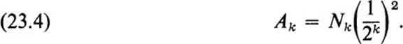
Then the number
![]()
is called the area of F.
Remark In Fig. 23.2 we have indicated for two successive values of k the operation described in Def. 23.3. Let us note that the quantity (l/2k)2 represents the value we would normally assign for the area of the squares (23.3) , and consequently the number Ak would correspond to the total area of those squares which lie inside F. Regardless of the geometric interpretation of Ak, the numbers Nk satisfy the relation Nk + 1 ≥ 4Nk, since to each square of the form (23.3) that lies in F correspond four squares of sides l/2k + 1, which lie in F. Therefore,

Thus the numbers Ak form a sequence in which each term is at least equal to or greater than the previous one. On the other hand, since by definition every figure F lies in some circle x2 + y2 ≤ R2, it also lies in a square − M ≤ x ≤ M, − M ≤ y ≤ M, for some integer M, and it follows that Ak ≤ (2M)2 for all k. It is a basic property of real numbers (see, for example, [3] Vol. I, Section 9.3) that the sequence Ak must then tend to a limit, so that the area as given by (23.5) is well defined for an arbitrary figure F. 4
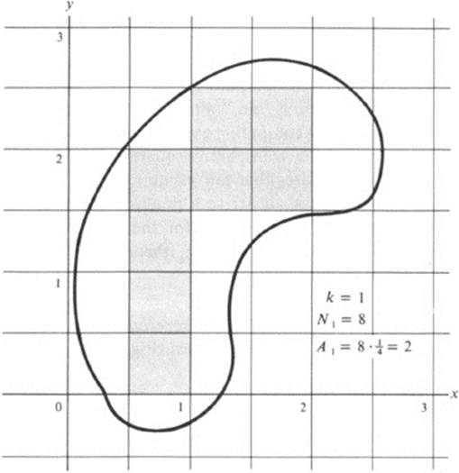
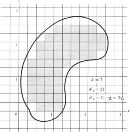
FIGURE 23.2 Illustration of the definition of area
There are two questions that must be asked about our definition (or for that matter, about any definition of area that is offered). The first is, “does it correspond to our intuitive notion of area?” and the second is, “can it be used practically to compute the area of a given figure?” The answer to the second question is “no,” although the definition does give an approximate value of area by computing explicitly a value of Ak. (This can be done in practice by placing a transparent square grid over the figure and counting the number of squares that fall inside.) On the other hand, using our definition as a basis, we shall derive a practical method for computing the area of many figures (Th. 23.3). As for the first question, it will be completely answered in the two following theorems. To state them, we introduce some useful terminology.
Definition 23.4 Two figures are said to overlap if they have at least one point in common other than boundary points ( Fig. 23.3).
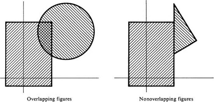
FIGURE 23.3 Distinction between overlapping and nonoverlapping figures
Definition 23.5 F is called the union of F1 …, Fn if the points of F consist of all points that lie in at least one of F1, …, Fn. We write F = Fx ∪. . .∪Fn ( Fig. 23.4).
Definition 23.6 A partition of a figure F is a collection of figures Fl…, Fn such that no two overlap, and F = Fx ∪. . . ∪ Fn ( Fig. 23.5).
Theorem 23.1 The notion of area introduced above has the following properties.
1. For every figure F, the area of F is a nonnegative real number.
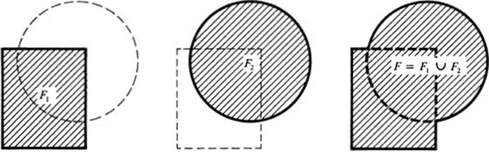
FIGURE 23.4 The union of two figures
2. If F1…, Fn form a partition of F, then the area of F is the sum of the areas of F1…, Fn.
3. If ![]() is obtained from F by a translation, then F and
is obtained from F by a translation, then F and ![]() have the same area.
have the same area.
4. If F is the square 0 ≤ x ≤ 1, 0 ≤ y ≤ 1, then the area of F is 1.
We do not give the details of the proof for this theorem. Let us note merely that properties 1 and 4 follow immediately from the definition, while properties 2 and 3 are considerably more difficult to prove. It is precisely in order to have property 2 that we so strictly limited the notion of a figure. In fact, if we apply our definition to more general point sets, property 2 need not hold at all (see Ex. 23.15).
The important fact to observe concerning Th. 23.1 is that the four properties listed are absolutely basic to our intuitive notion of area. Indeed, a careful examination of the elementary discussion given above, in deriving
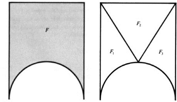
FIGURE 23.5 The partition of a figure
the formula for the area of a triangle, reveals that these four properties of area are used repeatedly in the reasoning, even though they are not explicitly stated. We could, of course, continue to list further basic properties of area, but that turns out to be unnecessary, in consequence of the following theorem.
Theorem 23.2 Suppose that to each figure F is assigned a real number A(F) such that the following conditions are satisfied:
1. For all F, A(F) ≥ 0.
2. If F1 .. ., Fn form a partition of F, then A(F) = A(F1) + (Fn).
3. If ![]() is obtained from F by a translation, then A(
is obtained from F by a translation, then A(![]() ) = A(F).
) = A(F).
4. If F is the square 0 ≤ x ≤ 1, 0 ≤ y ≤ 1, then A(F) = 1.
Then for every figure F, A(F) equals the area of F.
Once again, we omit the proof of this theorem (see, however, Ex. 23.13). The principal thing is to understand its content. We may summarize the situation as follows.
First, there is no unique way to define area. The particular definition we have given is one that seems intuitively reasonable and at the same time can be used to derive the four basic properties listed above.
Second, any other definition having these four properties must assign the same value for the area of an arbitrary figure as that obtained from our definition.
The next result is an illustration of how Th. 23.2 may be used.
Theorem 23.3 Let F be an arbitrary figure, and let L be any straight line. Let L(t) be the straight line parallel to L, at a distance | t | from L, where one side of the line L is chosen for positive values of t and the other side for negative values of t. Let h(t) denote the total length of those line segments on L(t) which lie in F (Fig. 23.6). Let a and b be any two numbers such that L(t) fails to meet F if t < a or if t > b. Then the area of F equals
PROOF. We indicate the proof only for polynomial figures. The same ideas apply in general, but there are some additional complications.5
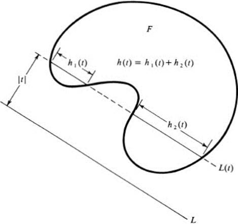
FIGURE 23.6 Notation for Th. 23.3
We consider a fixed line L, and we assign to each figure F the value6 of the integral (23.7), which we denote by A(F). In order to prove the theorem, it is sufficient to show that the number A(F) so defined verifies the four conditions of Th. 23.2. The first of these is obvious, since h(t) ≥ 0 for all t. For the second, we denote by h1(t),…, hn(t) the value of the function h(t) corresponding to the figures F1,…, Fn, respectively. Then, by the definition of a partition,
![]()
except in the case where the line L(t) contains a line segment that lies on the boundary of two distinct figures in the partition. However, assuming that F1, …, Fn are all polynomial figures, this can occur for at most a finite number of values of t. Thus Eq. (23.8) holds except for at most a finite number of values of t, and integrating (23.8) from a to b yields condition 2. Condition 3 is clear, since for the figure ![]() the corresponding function
the corresponding function ![]() (t) is of the form
(t) is of the form ![]() (t) = h(t + c) for a fixed constant c, and the integral (23.7) gives the same result for h(t) and
(t) = h(t + c) for a fixed constant c, and the integral (23.7) gives the same result for h(t) and ![]() (t). Finally, condition 4 may be verified by finding explicitly the function h(t) in this case, and carrying out the integration (23.7) (see Ex. 23.14).
(t). Finally, condition 4 may be verified by finding explicitly the function h(t) in this case, and carrying out the integration (23.7) (see Ex. 23.14). ![]()
Corollary 1 Let F be an arbitrary figure, and let ![]() be obtained from F by a rotation or a reflection. Then the area of
be obtained from F by a rotation or a reflection. Then the area of ![]() equals the area of F.
equals the area of F.
PROOF. In the case of a rotation, if the line L is subjected to the same rotation to yield a line ![]() , then the function
, then the function ![]() (t) corresponding to
(t) corresponding to ![]() and
and ![]() equals h(t) for all t, and the integral (23.7) yields the same value for both figures. In the case of a reflection, choose L to be the line in which the figure is reflected. Then
equals h(t) for all t, and the integral (23.7) yields the same value for both figures. In the case of a reflection, choose L to be the line in which the figure is reflected. Then ![]() (t) = h( − t), and again the integral is the same,
(t) = h( − t), and again the integral is the same, ![]()
Remark Clearly, a basic property we would expect from any reasonable definition of area would be invariance under all Euclidean motions. In the fundamental list of properties given in Th. 23.1 we only mentioned invariance under translation. We now see that it would have been superfluous to add invariance under rotation and reflection, since by Ths. 23.2 and 23.3 these are a consequence of the four stated properties, and indeed, must hold for any definition of area satisfying the conditions of Th. 23.2.
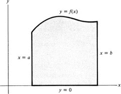
FIGURE 23.7 Area under a curve
Corollary 2 Let f(x) ∈ ![]() for a ≤ x ≤ b suppose f(x) > 0. Then the area of the figure (Fig. 23.7) defined by
for a ≤ x ≤ b suppose f(x) > 0. Then the area of the figure (Fig. 23.7) defined by
![]()
is equal to
![]()
PROOF. Note first that the point-set defined by (23.9) is indeed a figure in our sense. Its boundary consists of three line segments and a regular curve. If we choose the line L in Th. 23.3 to be the y axis, then t = x, h(t) = f(x), and (23.7) reduces to (23.10). ![]()
Remark In case f(x) is a polynomial, Eqs. (23.9) define a polynomial figure. This was the case for which we carried out the proof of Th. 23.3. Actually one can show that if f(x) is merely continuous, our definition of area gives the same value as the integral (23.10).
We may note that it is often the practice in elementary calculus not to define area, but to assume that it can be defined in a way that satisfies certain elementary properties (for example, if one figure is included in another, then the area of the first is less than or equal to that of the second), and to deduce from these properties that the integral (23.10) must represent the area. Thus, the discussion in the present section indicates one way to fill in the gap, by giving a definition of area having the necessary properties to obtain formula (23.10).
Exercises
23.1 Using the notation of Th. 23.3, let L be the y axis and let L(t) be the line x = t. Sketch each of the following figures F and find explicitly the function h(t).
a. F:x ≥ 0, y ≥ 0, x + y ≤ 1.
b. F: 2x − y ≥ 0, 2y + x ≥ 0, 2 − x ≥ 0
c. F: x − y ≥ 0, y − x2 ≥ 0
d. F:x + y ≥ 1, x2 + y2 ≤ 1
e. F:x2 + y2 ≤ 1, y − 2x2 + 1 ≥ 0
f. F:y (1 + x2)y ≤ 1, 2y − x2 ≥ 0
g. F:y ≤ ex, y ≥ e−x, x ≤ 2
h. F: y ≤ cos x, y ≥ sin x, x ≥ 0, x ≤ 1
i. F: 2x + y ≤ 2, y − 2x ≤ 2, y ≥ 0
j. F: | x |+ | y | ≤ 1
k. F: x + 3y ≥ 0, 3x − y ≥ 0, 2x + y ≤ 5
l. F: 4x − y2 ≥ 0, 2x − y ≤ 4
m. F: x2 + y2 ≤ 9,x2 + y2 ≥ 4
n. F: 2x − y2 ≥ 0, 4(x − 1) − y2 ≤ 0
o. F:x2 − 4 ≤ 0, y2 − 3y ≤ 0, 4x2 + y2 ≥ 4
*p. F:x2 + y2 ≤ a2, x2 ≤ b2; 0 < b ≤ a
23.2 Find the area of each figure in Ex. 23.1, using the value of h(t) obtained there and applying Th. 23.3. Check your answers, wherever possible, by means of standard expressions for area.
23.3 For each of the figures in Ex. 23.1, if L is the x axis, and L(t) is the line y = t, find the corresponding function h(t) (again in the notation of Th. 23.3).
23.4 Use the answers to Ex. 23.3 to compute the area of each figure in Ex. 23.1. Note that for a given figure, the choice of the line L can make a significant difference in the ease of computing the area.
23.5 Using the notation of Th. 23.3, let L be the line x + y = 0.
a. What is the equation of the line L(t)?
b. Find the function h(t) for the figure of Ex. 23.1a, and use it to compute the area.
c. Answer part b for the figure of Ex. 23.1j.
d. Answer part b for the figure of Ex. 23.1m.
23.6 Let F be the figure of Ex. 23.1a.
a. Sketch the figure F and the first three steps in the definition of the area of F (in analogy with Fig. 23.2).
b. Using the notation in the definition of area, compute the quantities N1, N2, N3, A1, A2, A3 for this particular figure.
*c. Find Nk and Ak for arbitrary k for this figure.
d. Use the answer to part c to obtain the area of F by direct use of the definition.
23.7 Which of the figures in Ex. 23.1 are polynomial figures?
23.8 Sketch the figure bounded by the right-hand loop of the curve y2 = x2(l − x2) and find its area.
*23.9 Sketch the figure bounded by the astroid x2/3 + y2/3 = a2/3, and find its area.
23.10 Note that in the definition of a polynomial figure, it is assumed first that the set of points is a figure, and second, that it is defined by a set of polynomial inequalities. In general, a set of points defined by polynomial inequalities need not be a figure. Show this in the following cases, by sketching the point sets described, and explaining carefully why each one fails to be a figure.
a. x2 + y2 − 1 ≥ 0
b. (x2 − y2)2 ≥ 0
c. −(x2 − y2)2 ≥ 0
d. −(x2 + y2 − l)2 ≥ 0
e. x2 − 1 ≥ 0, 4 − x2 − y2 ≥ 0
23.11 a. Draw a regular hexagon and sketch a partition of it using seven triangles.
b. Draw a square and sketch a partition of it using five rectangles.
*c. Find a partition of a square using six squares.
*d. Sketch a partition of a circle using two congruent figures with no straight-line segments in their boundaries.
23.12 Go over the elementary discussion of area which we used to introduce the subject, and note each place that one of the four properties given in Th. 23.1 was used.
*23.13 Carry out the following steps toward proving Th. 23.2.
a. Using properties 2, 3, and 4 in Th. 23.2, show that if Fmn is the figure defined by Eqs. (23.3), then A(Fmn) = (l/2k)2.
b. Given a figure F, consider for each integer k the partition of F into the squares Fmn of part a that lie inside F, and a remaining figure Fk, which is bounded by the boundary of F and parts of the boundaries of the squares Fmn. Draw a sketch indicating the figure Fk.
c. Using property 2 in Th. 23.2, together with part a, show that
![]()
where Ak is defined by Eq. (23.4).
d. Deduce that A(F) ≥ A, where A is the area of F. Note that in order to complete the proof of Th. 23.2, it is necessary to show that
![]()
It is here that some limitation is needed on the regularity of the boundary such as the condition we imposed in the definition of a figure.
23.14 The last step in the proof of Th. 23.3 requires finding the function h(t) and evaluating the integral (23.7) for the square F:0 ≤ x ≤ 1, 0 ≤ y ≤ 1, using an arbitrary straight line L. Carry out this computation for the following choices of the line L.
a. y = x
b. x + y = 0
*c. y = mx, where 0 < m < 1
*23.15 Let F be the square 0 ≤ x ≤ 1, 0 ≤ y ≤ 1. Let F1 consist of all those points (x, y) of F for which x is a rational number. Let F2 consist of all those points of F for which x is irrational. (Thus F1 and F2 are both made up out of vertical line segments.)
a. Show that F = F1 ∪ F2 and that F1and F2 have no points in common. (Thus, if F1 and F2 were figures, they would form a partition of F.)
b. Show that if the definition of area is applied to each of the sets F1 and F2, then the value obtained is zero. (In the terminology referred to in footnote 4 of this chapter, the “inner area” of F1 and of F2 is zero.) Since the area of F is equal to 1, property 2 of Th. 23.1 fails to hold in this generality.
*23.16 Let F be an arbitrary bounded set of points in the plane. Let Mk be the number of squares of the form defined by Eq. (23.3), which meet the figure F in at least one point. Let Bk = Mk(l/2k)2.
a. Show that Bk + 1 ≤ Bk for each k.
b. Show that Mk ≥ Nk for each k.
c. Deduce that the numbers Bk tend to a limit B, and that B ≥ A, where A is defined by Eq. (23.5).
(Note: the number B is called the outer area of the set F If B = A, their common value is called the area of F. In other words, every bounded set of points in the plane has a well-defined outer area and inner area. When the two coincide, their common value is defined to be the area. It is not hard to show that for a given set F, the outer area equals the inner area if and only if the boundary of F has zero area. It can also be shown that a piecewise smooth curve has zero area. Thus, for the sets we have denoted as “figures,” the quantity that we have defined to be area (and which is generally known as the inner area) coincides with the outer area and with the value of area defined more generally by the method indicated here.)