Two-Dimensional Calculus (2011)

Chapter 1. Background

3. Functions of two variables

The following are some typical examples of functions of two variables.

The first two examples are polynomials. A polynomial in two variables is the sum of terms of the form ax^myⁿ, where a is a constant, and m, n are nonnegative integers. The number m 4- n is called the degree of this term. The degree of a polynomial is the highest degree of the terms it contains. A polynomial is called homogeneous if all terms have the same degree. Thus example 2 above is a homogeneous quadratic polynomial (degree 2), while the most general homogeneous cubic polynomial is

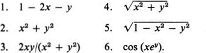
In studying functions of one variable, one can often gain a great deal of insight by associating with the function f(x) its graph, consisting of those points in the x, y plane for which y = f(x) (Fig. 3.1).

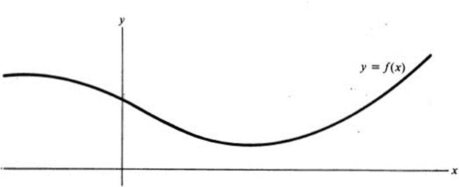
FIGURE 3.1 Graph of the function f(x)

An analogous procedure exists for visualizing a function f(x, y) of two variables. Associated with this function is the surface z = f(x, y) in 3-space. We illustrate this for each of the functions listed above.

Example 3.1

This is a linear equation, and hence represents a plane. (In analytic geometry one would write it in the form 2x + y + z = 1.) It intersects the z axis at the point where x and y are both zero, namely z = 1. Similarly, setting y = z = 0 yields x = , and x = z = 0 gives y = 1. These three points uniquely determine the plane (Fig. 3.2).

FIGURE 3.2 Plane

Example 3.2

This is the equation of a surface of revolution, since the value of z depends only on the distance (x² + y²)^1/2 from the z axis. If one uses polar coordinates, x = r cos θ, y = r sin θ, in the x, y plane, then the surface is given by the equation z = r². This is a paraboloid of revolution (Fig. 3.3).

Example 3.3

An important difference between this example and the previous ones is that the first two functions were defined for all values of x and y, whereas this one is not. More generally, every polynomial P(x, y) is defined for all x and y, whereas the quotient of two polynomials P(x, y)/Q(x, y) is undefined at points where the denominator vanishes. In this example the denominator vanishes at a single point, the origin, and hence this function is defined everywhere in the plane except at the origin. At the origin the numerator also vanishes, and it is not immediately clear how this function behaves near the origin. As in the previous example, the

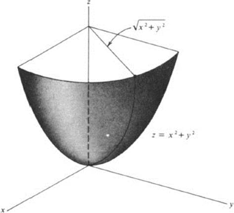
FIGURE 3.3 Paraboloid

introduction of polar coordinates in the x, y plane is helpful. Setting x = r cos θ, y = r sin θ, we find

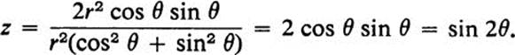
First we note that the value of z depends only on the polar angle θ and not on r. This means that z is constant on each ray θ = constant, or that the surface defined by z = sin 2θ contains a horizontal ray over each of these rays in the x, y plane. Second, we observe that the value of z always stays between +1 and − 1, so that the whole surface lies between the planes z = 1 and z = − 1. Finally, we see that as θ goes from 0 to π, z goes from 0 to 1, so that the surface is a kind of spiral ramp generated by starting with a ray along the positive x axis and moving it upwards, while holding it horizontally, as we rotate it through half of the first quadrant (Fig. 3.4).

If we continue to rotate the ray from θ = π to θ = π, its height drops back down from 1 to 0, at which point it coincides with the positive y axis. In the second quadrant, for π < θ < π, we have z = sin 2θ < 0, and the line drops below the x, y plane, reaching its lowest point at θ = π, when z = −1, and then rising again until it coincides with the negative x axis. Finally, as θ goes from π to 2π, this pattern is repeated. The final surface is of undulating form, covering the whole x, y plane except the origin.

Example 3.4

Once again it is easiest to use polar coordinates. We simply obtain z = r, which

FIGURE 3.4 “Spiral ramp” surface

represents a cone with vertex at the origin (Fig. 3.5). In contrast to the previous example, this function is defined for all values of x and y, although the resulting surface is clearly not “smooth” at the origin.

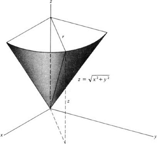
FIGURE 3.5 Cone

Example 3.5

Squaring both sides, we find z² = 1 − x² − y² or x² + y² + z² = 1. Thus all points on this surface lie on the sphere of radius 1 about the origin. Conversely, every point on this sphere satisfies z² = 1 − x² − y² and hence either z = (1 – x²– y²)^1/2 or z = –(1 − x² − y²)^1/2. Thus our equation defines those points on the sphere for which z ≥ 0; in other words, the upper hemisphere. Unlike the previous example, this surface is perfectly smooth at the origin. However, we now have a new phenomenon; namely, the function is only defined in a limited portion of the plane. There are no points of the surface above points in the x, y plane lying outside the circle x² + y² = 1 (Fig. 3.6).

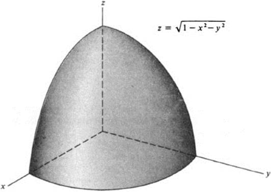
FIGURE 3.6 Sphere

Example 3.6

As in Example 3.3, we should probably note first that z takes on only values between 1 and −1; and hence the whole surface lies between the corresponding horizontal planes. To obtain an over-all picture, we might examine how this function behaves on each straight line y = c. We have then z = cos kx, where k is the positive constant e^c. In particular, along the x axis, where y = 0, we have z = cos x. For y < 0 we have k < 1, and we obtain a “stretched out” cosine curve, while for y > 0, we have k > 1, and hence a “compressed” cosine curve. Thus the undulations become more and more rapid on each line y = c as c → + ∞. It may help also to note that on the y axis, where x = 0, we have z = cos 0 ≡ 1. These features of the surface are illustrated in Fig. 3.7.

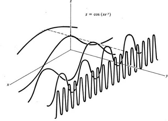
FIGURE 3.7 Cross sections of a surface

The following example, not included on our list at the beginning of this section, is of sufficient interest to warrant a separate discussion.

Example 3.7

We first try to determine the set of points in the x, y plane for which this function is defined. The quantity under the square root sign must be nonnegative, that is,

and

or using polar coordinates in the x, y plane

This says simply

which describes all points between the circles of radius 1 and 3 about the origin (Fig. 3.8).

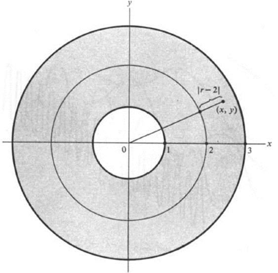
FIGURE 3.8 Set of points where a function is defined

We note next that z depends only on r, and not on θ, so that we have a surface of revolution whose intersection with each vertical plane through the z axis yields the same curve. Thus, in order to know the whole surface, it is sufficient to find its intersection with one half of the x, z plane, say x ≥ 0, y = 0. We have then

which is the upper half of the circle (Fig. 3.9)

or

Rotation about the z axis gives the upper half of a doughnut-shaped surface (Fig. 3.10). The entire surface is called a torus.

The above examples illustrate some of the methods by which we may obtain a geometric picture of a surface defined by a given function f(x, y). One way, as in Example 3.6, was to choose various values for y, and find the

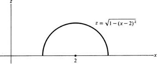
FIGURE 3.9 Cross section of a surface of revolution

curves on the surface that correspond to each of these values of y. In other words, find the intersection of the surface with vertical planes y = c for various values of the constant c. Similarly, we can pick values for x and see how f(x, y) behaves with respect to y, or we can introduce polar coordinates and study the function for values of r or θ. These are all special cases of the following general principle. If we are given a function f(x, y) and if we choose a straight line or curve in the x, y plane, then setting z = f(x, y) defines another curve lying over the given one. By choosing a suitable family of curves in the plane and constructing the corresponding curves on the surface, we may be able to visualize the entire surface.

There is a kind of inverse process to this one, which is also frequently of value. Instead of starting with curves in the x, y plane, we start with a fixed value of z and ask for those points in the x, y plane for which the function takes on the given value. In general, the set of points (x, y) for which f(x, y) = c, where c is any constant, is called a level curve of the function f(x, y). By choosing various values of c, and constructing the corresponding level curves, we can often quickly obtain a picture of the entire function. It may also be helpful to shade in those portions of the plane where f(x, y)

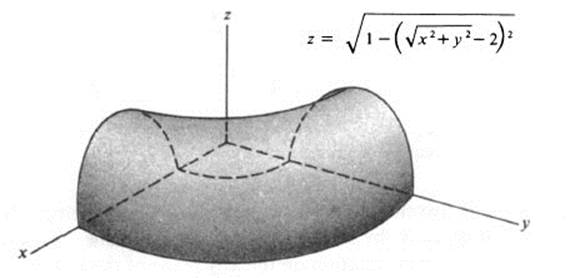
FIGURE 3.10 Torus

is positive. The corresponding surface z = f(x, y) then lies above the x, y plane in the shaded portions and below it in the unshaded portions.

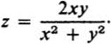
Example 3.8

The level curves xy = c are hyperbolas if c ≠ 0. For c positive, they lie in the first and third quadrants, while for c negative, they lie in the second and fourth quadrants. The level curve xy = 0 consists of the x and y axes (Fig. 3.11). This gives us a reasonably good over-all description of the function. It is zero at the origin, increases as we move out in either direction along the line y = x, and decreases in both directions along the line y = −x. On the basis of Fig. 3.11 it is easy to visualize the surface z = xy (Fig. 3.12). It is a “saddle-shaped” surface.

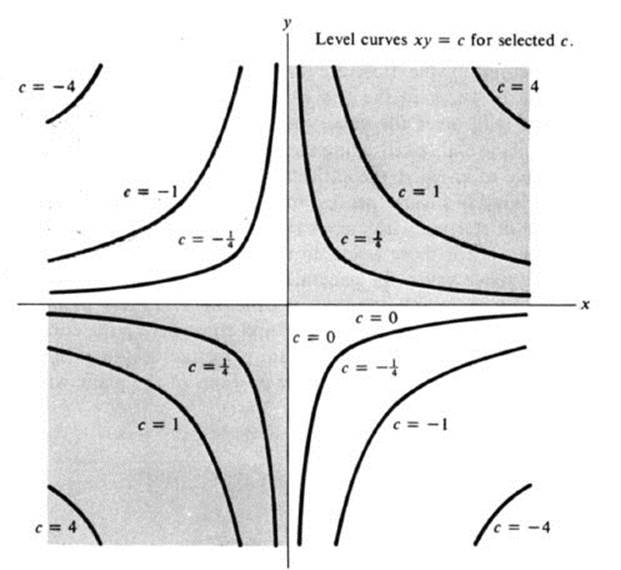
FIGURE 3.11 Level curves of the function xy

The relation between the above two methods of visualizing a function—by a surface in space or by level curves in the x, y plane—is clear; a level curve f(x, y) — c is the projection on the x, y plane of the intersection of the surface z = f(x, y) with a horizontal plane z = c (Fig. 3.13). This relation

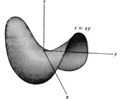
FIGURE 3.12 Surface z = xy

becomes more striking if we use the alternative expression “contour lines” for level curves. A contour line (or level curve) corresponds to the points on the surface z = f(x, y), which are at a given height above the x, y plane. A “contour map,” in the usual sense, gives a set of such curves when the function f(x, y) is the altitude above sea level. We may picture each function f(x, y) as defining a mountainous terrain, and our description of f(x, y) by level curves is simply a contour map to help guide us through the terrain.

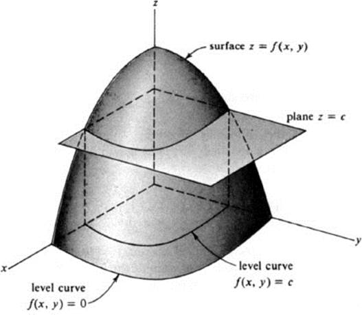
FIGURE 3.13 Level curves and horizontal cross sections

Exercises

3.1 Draw the intersection of each of the following surfaces with vertical planes y = c for various values of the constant c, and use these, as in Example 3.6, to visualize and sketch the entire surface.

a. z = xy

b. z = x² − y²

c. z = x² − 4y²

d. z = xy²

e. z = x/y

f. z = sin (x + y)

g. z = sin x sin y

h. z = ye^x

3.2 Study the surfaces in Ex. 3.1, using their intersections with vertical planes x = c for various values of c.

3.3 Draw a number of level curves for each of the functions in Ex. 3.1.

3.4 Using any or all of the devices in Exs. 3.1−3.3, try to visualize and sketch each of the following standard quadric surfaces. (Note: A, B, C are arbitrary positive constants. It may be easier in some cases to start by choosing two of these constants equal in order to obtain a surface of revolution.)

a.

b.

c.

*d.

*e.

3.5 For each of the following functions f(x, y), draw the level curve f(x, y) = 0, shade in the region where f(x, y) > 0, and try to visualize the surface z = f(x, y) near the origin.

a. x + y²

b. x² + 2xy + y²

c. x² + xy + y²

d. x² + 3xy + y²

e. x³ − 3xy²

f. x⁶ − yx² − yx⁴ + y²

3.6 Let a, b be a unit vector, and let x = at, y = bt be the line through the origin in the direction of that vector. For each of the functions f(x, y) of Ex. 3.5, sketch the curve on the surface lying above the given line. (In other words, substitute x = at, y = bt in the equation z = f(x, y) and find z as a function of t.) Try to picture how these curves vary as the vector a, b is changed, and use them to help visualize the surface.

3.7 If a function f(x, y) is of the form f(x, y) = g(x) + h(y), then the surface z = f(x, y) is called a surface of translation.

a. Explain this terminology by observing the cross sections of the surface z = f(x, y) with an arbitrary plane y = c, and the way these cross sections vary as c varies.

b. Do the same for the cross sections with planes of the form x = c.

c. Find which of the surfaces in the previous exercises are surfaces of translation, and illustrate this fact with corresponding sketches.

d. If either g or h is constant, the surface is called cylindrical. Describe what this means geometrically, and give some examples.

3.8 Let z = F(x), 0 < a ≤ x ≤ b, define a curve in the x, z plane. The surface defined by revolving this curve about the z axis is a surface of revolution.

a. What is the equation of the surface obtained in this way? (That is, if the surface is z = f(x, y), how is f(x, y) expressed in terms of the function F?)

b. What is the set of points in the x, y plane for which the function f(x, y) is defined?

c. What are the level curves of the function f(x, y)?

3.9 Describe geometrically how a surface z = f(x, y) would have to be transformed in order to obtain each of the following surfaces z = g(x, y), where g(x, y) is:

a. f(x, y) + 2

b. f(x + 2, y)

c. f(x, y − 2)

d. 2 − f(x, y)

e. f(− x, y)

f. 2f(x, y)

g. f(2x, y)

h. 2f( x, y)

i. −f(−x, −y)

j. f(y, x)

3.10 Let h(t) be a strictly increasing function of t, and let g(x, y) = h(f(x, y)).

a. How are the level curves of f(x, y) and g(x, y) related?

b. How is the surface z = g(x, y) related to the surface z = f(x, y)?

3.11 If the temperature at different points on the earth’s surface is considered a function of position, then the level curves of this function are called isotherms. (Either the temperature at a given time or the average temperature over some period may be used.) Figure 3.14 shows such a set of level curves for July temperatures in North America. Find approximately those points on the map where the following conditions prevail:

a. the temperature is maximum

b. the temperature is maximum relative to nearby points

c. the temperature changes most rapidly with respect to nearby points.

3.12 Figure 3.15 is a portion of a contour map showing two mountain streams running vertically and a connecting stream between them.

a. Find approximately the point where the terrain is steepest.

*b. By examining the contour lines determine the direction of flow of each of the three streams.

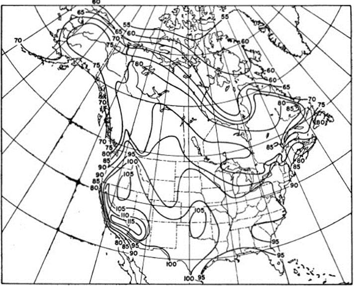
FIGURE 3.14 Isotherms for July temperatures

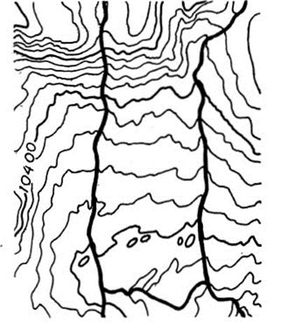
FIGURE 3.15 Portion of a contour map [U.S. Geological Survey topographic map.]

¹ For further discussion of vectors from various points of view, see [5], [9], and [10].

2 It may be argued that our definition of a curve is somewhat ambiguous, since it essentially describes how a curve is represented without stating clearly what a curve is. A reader who is bothered by this lack of precision may find it clearer to say that a curve is the pair of functions x(t), y(t). The remainder of the text may then be read without change. Although this way of gaining precision is frequently used, we have preferred a less formal formulation, which embodies the intuitive notion of what a curve consists of. This intuitive notion has in fact been made rigorous in a variety of ways, each one abstracting some particular aspect of curves. There are a number of current definitions of curves in different branches of modern mathematics. Thus, in differential geometry a curve is often defined by starting with pairs of functions x(t), y(t) and considering two pairs to be equivalent if one is obtained from the other by a suitable change of parameter. In algebraic geometry a curve is generally regarded as a set of points, corresponding to what we have called the “implicit form” of a curve. For more sophisticated discussions of curves from these two points of view see [17], pp. 1–6, and [35], Chapter 3.

³ See [14], Section 7.3, in which this is proved for nonparametric curves y = f(x), and see Exercise 2.18. Direct proofs may be found, for example, in [3], Vol. 1, Section 6.33, and in [27], Section 13.3. For a good review of parametric curves, and for further exercises, see Chapter 7 of [14].

⁴ Here we are implicitly using the fact that limit operations on vectors may be performed by carrying out the limit process on each component.

⁵ For a wealth of examples of plane curves, with illuminating discussions of each, see [24].

⁶ See, for example [14], p. 222. In the form given there, the rule actually applies to the reciprocal quantity 1/m(t), which tends to zero as t tends to zero.

⁷ See [12], where it is shown how Lissajous figures are used to determine frequency and phase differences.