Biology Premium, 2024: 5 Practice Tests + Comprehensive Review + Online Practice - Wuerth M. 2023

About the Exam
2 Statistics in AP Biology

Learning Objectives

In this chapter, you will learn:

➜What Is a Null Hypothesis?

➜Chi-Square Test

➜Descriptive Statistics

Overview

Scientists make hypotheses and then design experiments to test these hypotheses. Data are gathered during these experiments and then analyzed. Scientists use these analyses to draw conclusions about the data. An important tool in data analysis is statistics. Statistical tests are used to evaluate hypotheses. Descriptive statistics describe data sets. This chapter will review some of the statistical tests and descriptive statistics you need to understand for the AP Biology course and exam.

What Is a Null Hypothesis?

The null hypothesis (H₀) states that there is no statistically significant difference between two groups in an experiment. For example, a student designs an experiment to see if plants watered with bottled water will exhibit more growth than plants watered with tap water. The null hypothesis for this experiment would be that there will be no statistically significant difference in plant growth between the plants watered with bottled water and the plants watered with tap water.

Here’s another example: You want to test if dogs prefer dog food brand A over dog food brand B. The null hypothesis would be that there will be no statistically significant difference between the number of dogs choosing dog food brand A and the number of dogs choosing dog food brand B. If 100 dogs are presented with both dog food brand A and dog food brand B, the null hypothesis would predict that 50 dogs would choose brand A and 50 dogs would choose brand B.

Chi-Square Test

The chi-square test is a statistical test that is used to compare the observed results to the expected results in the experiment. In AP Biology, the chi-square test is used to evaluate the null hypothesis, and it is often used in genetics problems, in the lab on mitosis (Lab 7), and in the lab on animal behavior (Lab 12).

It is important to note that the chi-square test is used to compare primary or raw data, such as the number of items in each category of data. The chi-square test should not be used to compare processed data, such as percentages or means. For example, it would be appropriate to use the chi-square test if you were comparing the number of purple flowers and the number of white flowers that resulted from a genetic cross. It would not be appropriate to use the chi-square test to compare the percentage of purple flowers to the percentage of white flowers.

Consider the experiment that measured whether dogs prefer dog food brand A or dog food brand B. If there are 100 dogs, the null hypothesis would predict that 50 dogs would choose brand A and 50 dogs would choose brand B. These are the expected results. If the experiment was carried out and 45 dogs chose brand A and 55 dogs chose brand B, those are the observed results. The chi-square test could be used to evaluate the null hypothesis that there will be no statistically significant difference between the expected results and the observed results of the experiment. The steps of the chi-square test are as follows:

TIP

You do NOT need to memorize any of the formulas reviewed in this chapter—they are included on the AP Biology Equations and Formulas sheet, which will be supplied to you on test day. For quick reference, you can review those formulas in the Appendix of this book.

1.Calculate the chi-square value. The formula for chi-square is:

The symbol ∑ means “summation.” This means you need to do this calculation for each category of data (brand A and brand B) and then add the values.

Using the observed and expected values (45 observed and 50 expected for brand A; 55 observed and 50 expected for brand B):

2.Determine the number of degrees of freedom (df) in the experiment. The number of degrees of freedom in an experiment is defined as the number of possible outcomes in the experiment minus 1. In this experiment, there are two possible outcomes, brand A or brand B, so the df is 2 — 1 = 1.

3.Using the degrees of freedom and the p-value, find the critical value in the chi-square table. The p-value is defined as the probability that the observed data would be produced by random chance alone. For biology, the typical p-value used is 0.05. Using the df of 1 calculated above and a p-value of 0.05, the critical value is 3.84 according to the chi-square table that follows.

Chi-Square Table

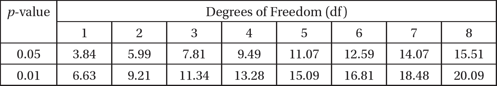
4.Compare your calculated chi-square value to the critical value. The calculated chi-square value from the first step (1) is less than the critical value (3.84).

5.Based on the comparison, decide whether to reject the null hypothesis or whether you fail to reject the null hypothesis. If the calculated chi-square value is less than or equal to the critical value, fail to reject the null hypothesis. If the calculated chi-square value is greater than the critical value, reject the null hypothesis.

In this example, since the calculated chi-square value is less than the critical value, you would fail to reject the null hypothesis that there is no statistically significant difference between the observed and expected data. This does not mean the null hypothesis is proven—it just means you cannot reject the null hypothesis. In other words, the null hypothesis cannot be ruled out.

Here is another example: A coin has heads on one side and tails on the other side. If the coin is flipped 40 times, you would expect the coin to come up heads 20 times and come up tails 20 times. These are the expected results. The coin is flipped 40 times, and the coin comes up heads 12 times and it comes up tails 28 times. Those are the observed results. The null hypothesis is that there is no statistically significant difference between the observed and expected numbers of heads and tails. To evaluate this null hypothesis, here are the steps involved:

1.Calculate the chi-square value.

2.Determine the number of degrees of freedom (df) in the experiment. There are two possible outcomes in this experiment (heads or tails), so the df is 2 — 1 = 1.

3.Using a df of 1 and a p-value of 0.05, the critical value is 3.84 according to the chi-square table.

4.Compare your calculated chi-square value to the critical value. The calculated chi-square value (6.40) is greater than the critical value (3.84).

5.Decide whether to reject the null hypothesis or whether you fail to reject the null hypothesis. In this example, you should reject the null hypothesis because the calculated chi-square value is greater than the critical value. Since the null hypothesis is rejected, you can then come up with an alternative hypothesis—for example, perhaps this is a “trick coin”!

Descriptive Statistics

Descriptive statistics are used to describe data sets. There are descriptive statistics that describe the center of a data set, and other descriptive statistics describe the amount of variability or spread of a data set.

The mean and median can be used to characterize the center of a data set. Thus, the mean and median are sometimes referred to as measures of the central tendency of a data set.

The mean, or average, of a data set is calculated with the following formula:

In the above formula:

n = sample size (the number of data points in the data set)

∑ = summation (add all members of the data set, starting with the first member of the set, and continue to the nth member of the data set)

x_i = the ith member of the data set

To calculate the mean, add the values of all the data points in the data set, and then divide that by the sample size. (Multiplying by gives the same result as dividing by n.) Here’s how you would calculate the means for data set A and data set B:

Data Set A: 1, 2, 3, 4, 5; n = 5

Data Set B: 3, 3, 3, 3, 3; n = 5

Notice that data set A looks very different from data set B, but they both have the same mean. Means can be distorted or skewed by extreme values in the data set. These two data sets illustrate how looking at just the mean is sometimes not enough to accurately describe the data set.

The median is the midpoint of the data set. To find the median, place the members of the data set in numerical order from lowest to highest value. The middle of the data set is the median. If there are an even number of data points in the set, calculate the mean of the two numbers in the middle of the data set to find the median. Here’s how you would find the median for data set A and data set B:

Data Set A: 1, 2, 3, 4, 5

Since the members of the data set are already arranged from lowest to highest, look for the middle value, which in this case is 3.

Data Set B: 3, 3, 3, 3, 3

Since the members of this data set are all the same, the median is 3.

Again, even though data sets A and B are very different, they have the same median.

Extremes in a data set do not affect the median, but they do affect the mean of the data set. For example, add the numbers 0 and 100 to data set A and data set B to form new data sets C and D, respectively. This changes the means greatly from the original calculations, but the medians do not change:

Data Set C: 0, 1, 2, 3, 4, 5, 100

Data Set D: 0, 3, 3, 3, 3, 3, 100

Using the mean and median alone are often not enough to accurately describe a data set. It is also important to use descriptive statistics that describe the spread of a data set. Standard deviation and standard error of the mean can be used to describe how spread out the data points are.

You will not be required to calculate standard deviation or standard error of the mean on the AP Biology exam. However, it is important to understand what standard deviation and standard error of the mean can tell you about a data set. You also must be able to use standard error of the mean to construct 95% confidence intervals.

Standard deviation (s) averages how far each data point is from the mean of the data set. The formula for standard deviation is:

Here’s how you would calculate the standard deviation for data set A and data set B:

Data Set A: 1, 2, 3, 4, 5; and n = 5

Data Set B: 3, 3, 3, 3, 3; and n = 5

If a data set is more spread out, the standard deviation will be larger. The less spread out the data points, the smaller the standard deviation.

The standard error of the mean is another measure of how spread out a data set is. Each time you repeat an experiment, random chance will lead to slightly different means. If an experiment is repeated multiple times and a mean is calculated for each experiment, the standard error of the mean predicts the distribution of the means of those repeated experiments. The prediction would be that 95% of the means would fall within two standard errors of the mean (above or below the mean of the original experiment). If the standard error of the mean is large, repeating the experiment will result in a larger range of means than if the standard error of the mean was small. Data sets with smaller standard errors of the mean are considered more accurate.

Standard error of the mean is calculated with the following formula:

In the above formula:

s = standard deviation

n = sample size

Notice that as the sample size (n) increases, the standard error of the mean decreases. You may already understand that an experiment performed with a larger sample size is considered more reliable than an experiment performed with a smaller sample size. Standard error of the mean gives a mathematical reason for why experiments with larger sample sizes are typically more reliable. Here’s how you would calculate the standard error of the mean for data set A and data set B:

Data Set A: 1, 2, 3, 4, 5; s = 1.58 and n = 5

Data Set B: 3, 3, 3, 3, 3; s = 0 and n = 5

Standard error of the mean can be used to create a type of error bar on a graph called a 95% confidence interval (95% CI). A 95% confidence interval does NOT mean you are 95% confident in your data! What a 95% confidence interval does mean is that if you repeated an experiment 100 times and calculated the mean of the data you collected each time, the mean would fall within the 95% confidence interval 95 of those 100 times. In other words, you would expect your mean to fall within the 95% confidence interval 95% of the time, but 5% of the time you would expect the mean to be outside of the 95% confidence interval.

To construct a 95% confidence interval, you need to know the upper limit of the interval and the lower limit of the interval. The upper limit of the 95% confidence interval is found by starting with the mean and then adding two times the standard error of the mean:

To find the lower limit of the 95% confidence interval, start with the mean and then subtract two times the standard error of the mean:

Here’s an example to practice working with 95% confidence intervals.

An AP Biology class grows “Fast Plants” (Brassica rapa) and records the height of each plant on day 28 of growth. The mean plant height and standard error of the mean are calculated. The 10 tallest plants are cross-pollinated and produce seeds. These seeds are harvested and planted to form a second generation of plants. The height of each plant in this second generation is measured, and again the mean plant height and standard error of the mean are calculated. The data are shown in the following table:

Construct a graph of the mean plant height for each generation, showing 95% confidence intervals. First, find the upper and lower limits for the 95% confidence intervals for each generation.

For Generation 1:

Upper limit of 95% CI = 158.4 + 2(8.8) = 176.0 mm

Lower limit of 95% CI = 158.4 — 2(8.8) = 140.8 mm

For Generation 2:

Upper limit of 95% CI = 203.1 + 2(9.6) = 222.3 mm

Lower limit of 95% CI = 203.1 — 2(9.6) = 183.9 mm

Graphing the means for each generation with the 95% confidence intervals leads to Figure 2.1.

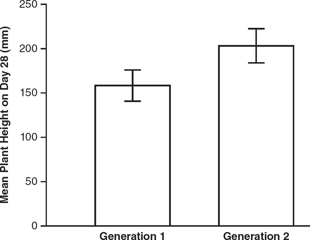
Figure 2.1 Mean Plant Height on Day 28 for Generations 1 and 2

Now that you know how to construct graphs with 95% confidence intervals, it is important to understand what they can tell us when comparing data sets. In the previous example, the 95% confidence intervals for generations 1 and 2 do not overlap. If the 95% confidence intervals for two sets of data do not overlap, it is likely there is a statistically significant difference between the two groups. In that example, there is likely a statistically significant difference between the mean plant heights on day 28 for generations 1 and 2.

However, if the 95% confidence intervals do overlap, the data are inconclusive, and it is not possible to say whether or not there is a significant difference between the groups. The experiment would need to be repeated. Here is another example that illustrates this point.

On field trips to a salt marsh, an AP Biology class counted the number of crustaceans in a 100 cm² quadrant. Three different locations in the marsh were visited, and multiple quadrants were counted at each location. The mean number of crustaceans per quadrant and the standard error of the mean were calculated from the data at each location. The data are shown in the following table.

The data from each location were plotted with 95% confidence intervals (calculated as follows). Figure 2.2 shows the graph of this data.

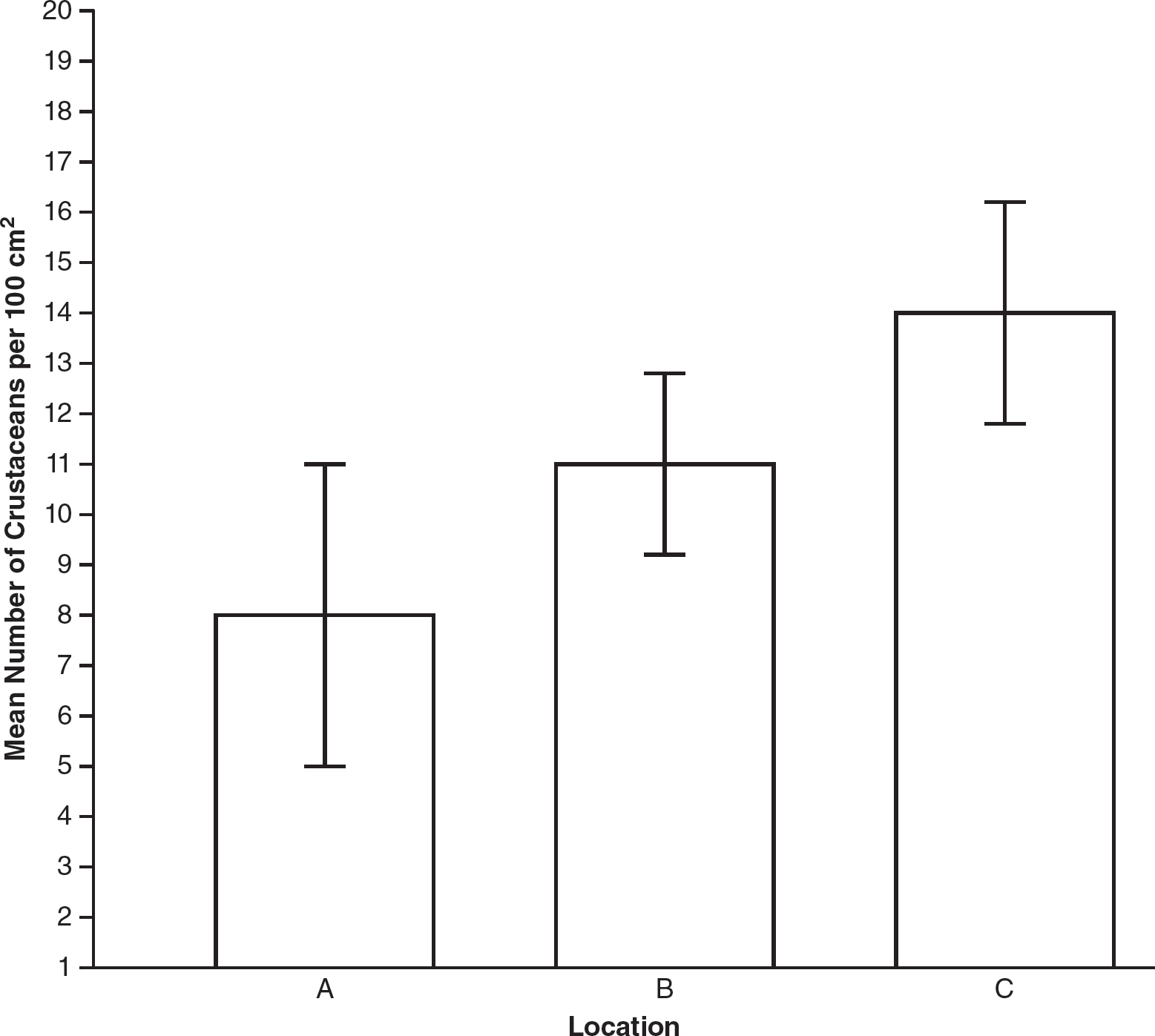
Figure 2.2 Mean Number of Crustaceans per 100 cm² in Three Locations in the Salt Marsh

Which of the two locations are most likely to have a statistically significant difference in the number of crustaceans found per 100 cm²? The answer is that locations A and C would most likely have statistically significant differences because the 95% confidence intervals for locations A and C do not overlap. The 95% confidence intervals for locations A and B do overlap, so it is not possible to make any conclusions about statistically significant differences between those two locations. Similarly, the 95% confidence intervals for locations B and C overlap, so it is also not possible to make any conclusions about statistically significant differences between locations B and C.

Practice Questions

Multiple-Choice

1.Which of the following can be used to describe the center of a data set and is NOT affected by extreme values in the data set?

(A)mean

(B)median

(C)standard deviation

(D)standard error of the mean

2.Data Set A consists of {10, 15, 15, 20, 25}. Data Set B consists of {15, 15, 17, 19, 19}. Which of the following descriptive statistics is the same for both data set A and data set B?

(A)mean

(B)median

(C)standard deviation

(D)standard error of the mean

3.The chi-square test is appropriate to compare which of the following types of data?

(A)means

(B)percentages

(C)processed data

(D)raw data

4.In a dihybrid cross of two organisms (AaBb × AaBb), four different phenotypes of offspring can be produced. How many degrees of freedom would there be?

(A)1

(B)2

(C)3

(D)4

5.In pea plants, the tall (T) allele is dominant to the dwarf (t) allele. Two heterozygous (Tt) pea plants are crossed and produce 400 offspring. Three hundred offspring are expected to be tall, and 100 are expected to be short. There are 290 tall offspring observed and 110 dwarf offspring observed. Calculate the chi-square value from this data (using a p-value of 0.05), and state whether there is likely a statistically significant difference between the observed and expected data.

(A)The chi-square value is 0.67. There is a statistically significant difference between the observed and expected data.

(B)The chi-square value is 0.67. There is NOT a statistically significant difference between the observed and expected data.

(C)The chi-square value is 1.33. There is a statistically significant difference between the observed and expected data.

(D)The chi-square value is 1.33. There is NOT a statistically significant difference between the observed and expected data.

6.A student wanted to see if isopods preferred banana or watermelon as a food source. Twenty isopods were placed in the center of a choice chamber with two compartments. Banana was placed in one compartment, and watermelon was placed in the second compartment. After 15 minutes, the number of isopods in each compartment was counted. Data are shown in the table.

The null hypothesis was that the isopods would have no food preference and would be found in equal numbers in both compartments. Calculate the chi-square value (using a p-value of 0.05), and determine if there was a statistically significant difference between the observed and expected data in this experiment.

(A)The chi-square value is 0.80. There is a statistically significant difference between the observed and expected data.

(B)The chi-square value is 0.80. There is NOT a statistically significant difference between the observed and expected data.

(C)The chi-square value is 3.20. There is a statistically significant difference between the observed and expected data.

(D)The chi-square value is 3.20. There is NOT a statistically significant difference between the observed and expected data.

7.Data Set X and Data Set Y have the same standard deviations. Data Set X has a sample size of 10, while Data Set Y has a sample size of 50. How will their standard errors of the mean compare?

(A)Data Set X will have a larger standard error of the mean than Data Set Y.

(B)Data Set Y will have a larger standard error of the mean than Data Set X.

(C)Both data sets will have the same standard error of the mean.

(D)The difference in the standard errors of the mean cannot be determined from the information given.

Questions 8 and 9

The heights of oak trees in four different locations were measured. The mean height and the standard error of the means were calculated for each location and are shown in the table.

8.Which location showed the greatest variability in the heights of the oak trees?

(A)Oakville

(B)Sacramento

(C)San Rafael

(D)Oak Valley

9.Which of the following two locations are likely to have a statistically significant difference between the heights of their oak trees?

(A)Oakville and Sacramento

(B)Oakville and Oak Valley

(C)San Rafael and Oak Valley

(D)San Rafael and Oakville

10.Which of the following correctly describes how to calculate a 95% confidence interval?

(A)Mean ± 1(Standard Deviation)

(B)Mean ± 1(Standard Error of the Mean)

(C)Mean ± 2(Standard Deviation)

(D)Mean ± 2(Standard Error of the Mean)

Short Free-Response

11.Some chemicals are known to increase the frequency of chromosome breakage in dividing cells. Thirty Petri dishes with dividing cells were treated with either lead (10 Petri dishes), cadmium (10 Petri dishes), or control solutions (10 Petri dishes). Forty-eight hours after treatment, each Petri dish was examined, and the percentage of cells that showed chromosome breakage in each Petri dish was calculated. The mean percentage of cells that showed chromosome breakage and the standard error of the mean for each treatment were calculated and are shown in the table.

(a)Describe which treatment produced the greatest variability in the data.

(b)Describe which treatment was least likely to result in chromosome breakage.

(c)A student claims that exposure to cadmium is more likely to result in chromosome breakage than exposure to lead. Evaluate this claim using the data provided.

(d)Identify the independent variable and the dependent variable in this experiment.

12.In tobacco plants, green (G) is dominant to albino (g). A heterozygous green (Gg) tobacco plant is crossed with an albino (gg) tobacco plant, and 100 offspring are produced. Fifty offspring are expected to be green (Gg), and 50 offspring are expected to be albino (gg). However, when the offspring are counted, 60 green plants and 40 albino plants are observed.

(a)Identify the degrees of freedom in this experiment.

(b)Calculate the chi-square value for this data.

(c)Make a claim about whether or not the observed data are likely significantly different statistically from the expected data. Use a p-value of 0.05.

(d)Justify your claim from part (c) with your knowledge of the chi-square test.

Long Free-Response

13.Organic gardeners will sometimes use ladybugs as a method of reducing aphid populations in their gardens. A garden infested with aphids is divided into three sections. In the first section, no treatment (to reduce the aphid populations) is applied. In the second section, ladybugs are introduced to reduce the aphid populations. In the third section, a chemical pesticide is used to reduce the aphid populations. One week after the treatments are applied, 10 measurements of the density of the aphid populations (in aphids per square decimeter) are taken in each section of the garden. The means and the 95% confidence intervals for each section of the garden are shown in the graph.

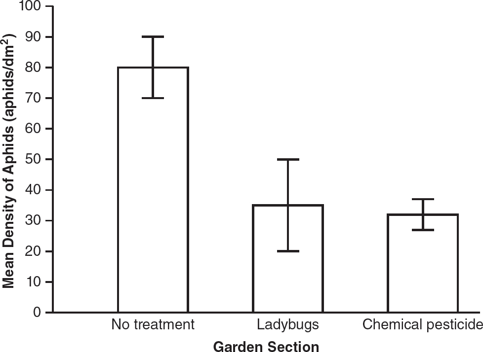
(a)Based on the graph, identify the section of the garden with the least variability in aphid density and the section of the garden with the most variability in aphid density one week after treatment.

(b)Analyze the data shown in the graph to determine which sections of the garden are most likely to have a statistically significant difference in aphid density.

(c)In this experiment, 10 measurements (n = 10) of the aphid density were taken in each section of the garden. If 50 measurements (n = 50) were taken, make a prediction about the effect, if any, this would have on the 95% confidence intervals.

(d)Justify your prediction from part (c) using your knowledge of how 95% confidence intervals are calculated.

Answer Explanations

Multiple-Choice

1.(B)The median is the midpoint of a data set and is not as affected by extreme values in a data set in the same way that the mean is. Extreme values in a data set skew the mean, so choice (A) is incorrect. The mean is used to calculate standard deviation, so standard deviation would be affected by extreme values in a data set. Thus, choice (C) is incorrect. Choice (D) is incorrect because standard error of the mean is also affected by extreme values in a data set.

2.(A)The mean for both data sets is 17. Choice (B) is incorrect because the median for data set A is 15, while the median for data set B is 17. The spread for data set A (25 — 10 = 15) is larger than the spread for data set B (19 — 15 = 4), so the standard deviation and the standard error of the means for those data sets will likely be different. Therefore, choices (C) and (D) are incorrect.

3.(D)The chi-square test is most appropriately used on raw data, such as the numbers of individuals in each category. The values used in the chi-square table have been calculated by statisticians and are designed to be used with raw data. Processed data, such as means and percentages, cannot be used with the chi-square test, making choices (A), (B), and (C) incorrect.

4.(C)Since there are four different phenotypes that could be produced, there are 3 degrees of freedom. Degrees of freedom = number of possible outcomes in the experiment — 1 = 4 — 1 = 3.

5.(D). Using the observed and expected values in the problem:

. There are two possible outcomes in the experiment (tall or dwarf), so the degrees of freedom = 2 — 1 = 1. Using the p-value of 0.05 and the chi-square table, the critical value is 3.84. The calculated chi-square value from the data is less than the critical value, so there is likely no statistically significant difference between the observed data and the expected data. Choices (A) and (B) are incorrect because they have incorrect calculations of the chi-square data. Choice (C) is incorrect because even though the chi-square value from the data is calculated correctly, the wrong conclusion is drawn from the result.

6.(D)The chi-square . There are two possible outcomes in the experiment (banana or watermelon), so there is one degree of freedom. Using the p-value of 0.05 and the chi-square table, the critical value is 3.84. The calculated chi-square value is less than the critical value, so there is likely not a statistically significant difference between the observed and expected data. Choices (A), (B), and (C) are incorrect because they present the wrong chi-square value and/or the wrong conclusion about the data.

7.(A)Standard error of the mean is calculated by dividing the standard deviation by the square root of the sample size . If the standard deviation is the same for both data sets, the standard error of the mean will decrease when the sample size increases. Since both data sets have the same standard deviation, the data set with the smaller sample size (Data Set X, which has n = 10) will have a larger standard error of the mean than Data Set Y, which has a larger sample size (n = 50).

8.(C)The standard error of the mean is a way to measure the variability or spread of a data set. The larger the standard error of the mean, the greater the variability in the data set. Since data collected in San Rafael has the highest standard error of the mean, San Rafael has the greatest variability in the data.

9.(B)The upper limit of the 95% confidence interval for data from Oakville (25.1) is less than the lower limit of the 95% confidence interval for data from Oak Valley (30.1). So their 95% confidence intervals do not overlap and there is likely a significant difference between the oak tree heights in those two locations. Choice (A) is incorrect because the 95% confidence interval for the data from Sacramento overlaps with the 95% confidence interval for the data from Oakville (the upper limit for Sacramento of 19.6 is greater than the lower limit for Oakville of 15.1). Similarly, the 95% confidence intervals for data from San Rafael and Oak Valley overlap (the upper limit for San Rafael of 37.3 is greater than the lower limit for Oak Valley of 30.1), so choice (C) is incorrect. Choice (D) is incorrect because the 95% confidence intervals for data from San Rafael and Oakville overlap (the upper limit for Oakville of 25.1 is greater than the lower limit for San Rafael of 20.1).

10.(D)The upper limit of a 95% confidence interval is determined by adding two times the standard error of the mean to the mean of the data set, which is represented by choice (D). The lower limit of the 95% confidence interval is determined by subtracting two times the standard error of the mean from the mean of the data set. Choices (A), (B), and (C) are incorrect because they do not represent the upper limit or the lower limit of a 95% confidence interval.

Short Free-Response

11.(a)The treatment with cadmium resulted in the greatest variability in the data because it has the greatest standard error of the mean.

(b)The control treatment was the least likely to result in chromosome breakage. Its mean percentage of cells that showed chromosome breakage was far lower than the mean for the other two treatments.

(c)The upper limit of the 95% confidence interval for lead (24.3 + 2(5.2) = 34.7) is greater than the lower limit of the 95% confidence interval for cadmium (46.1 — 2(9.1) = 27.9), so the 95% confidence intervals for those two treatments overlap. When the 95% confidence intervals overlap, the data are inconclusive and it is not possible to claim that there is a statistically significant difference between the groups. The data provided do not support the student’s claim that cadmium is more likely to result in chromosome breakage than exposure to lead.

(d)The independent variable is the type of treatment (control, lead, or cadmium). The dependent variable is the mean percentage of cells that showed chromosome breakage.

12.(a)There are two possible outcomes in this experiment (green or albino), so the number of degrees of freedom (df) = 2 — 1 = 1.

(b)

(c)The observed data are likely statistically significantly different from the expected data.

(d)With one degree of freedom and using a p-value of 0.05, the critical value from the chi-square table is 3.84. Since the calculated chi-square value (4) is greater than the critical value, there is likely a statistically significant difference between the observed and expected values.

Long Free-Response

13.(a)The section of the garden with the least variability in aphid density is the section treated with chemical pesticide because its 95% confidence interval is the smallest. The section with the most variability is the section treated with ladybugs because its 95% confidence interval is the largest.

(b)The 95% confidence interval for the section that received no treatment does not overlap with the 95% confidence intervals for the ladybug section or the chemical pesticide section. Thus, the section that received no treatment is least like the others and is most likely to have a statistically significant difference in aphid density from the ladybug- and chemical pesticide—treated sections.

(c)If 50 measurements were taken in each section, the 95% confidence intervals would be smaller.

(d)To calculate 95% confidence intervals, add or subtract two times the standard error of the mean from the mean of the data set. The standard error of the mean is inversely proportional to the sample size (if the sample size increases, the standard error of the mean decreases). So if the sample size, n, increased to 50 for all three sections, the standard errors of the mean for each section would likely decrease, and the 95% confidence intervals would be smaller.