Botany: An Introduction to Plant Biology - Mauseth, James D. 2017
Ecology
Community Ecology
Chapter Opener Image: The art above illustrates a food web within a community. All organisms are interconnected in that some (especially plants) are the food for others (animals, fungi and bacteria). Plants do not eat each other, of course, but they might interact indirectly in that if one species is present, an animal prefers to eat it and leaves other species of plants alone, whereas if the first is not present, then the animal eats other, less desirable plants. Alternatively, the presence of one species might be so nutritious that the animal population increases and they then inadvertently trample other plants.
OUTLINE
✵ Concepts
✵ Diversity
- Diversity and Scale
- Diversity and Latitude
✵ Predator—Prey Interactions
- One Predator, One Prey
- Predator Selection Among Multiple Prey
- Competition Between Species
- Apparent Competition
✵ Beneficial Interactions Between Species
✵ Metapopulations in Patchy Environments
✵ Interconnectedness of Species: Food Chains and Food Webs
Box 26-1 Plants Do Things Differently: Plants and Animals Are Different Kinds of Prey
Box 26-2 Plants and People: Some Laws to Protect Species Have Harmful Consequences
LEARNING OBJECTIVES
After reading this chapter, students will be able to:
✵ State the importance of studying community ecology.
✵ List three ways to measure community diversity.
✵ Recall the species—area relationship (formula).
✵ Identify two hypotheses that seek to explain why there is more organism diversity in tropical climates as compared to cooler climates.
✵ Explain predator—prey cycling in a one predator—one prey scenario.
✵ Give an example of the paradox of enrichment.
✵ Define maximum sustained yield and describe how it affects our use of natural resources such as forests and oceans.
✵ List three factors affecting a predator’s choice of prey.
✵ Explain mutualism and facilitation and give an example of each.
✵ Discuss migration corridors and their importance in our efforts to protect endangered species.
✵ Define keystone species and give an example of how removal or reintroduction can affect a community.
 Did You Know?
✵ All individual organisms are members of a community, which consists of all the individuals that live at the same time and place.
✵ We humans are members of any community where we live, hunt, fish, mine minerals, or otherwise affect other organisms.
✵ Any natural area, no matter how rich its diversity, lacks thousands of species that cannot compete against the organisms that are already present.
✵ Many plants, animals, and microbes help each other in pollination and nitrogen fixation, but only so long as it is beneficial to each.
✵ Wildlife preserves designed to help a particular species must also help all the community members on which that species depends.
![]() Concepts
Concepts
A community is a group of species that occur together at the same time and place (FIGURES 26-1 and 26-2). Population biology focuses on the members of a single species, their growth, interbreeding, survival, and so on. Community ecology might examine that same species but would take into consideration its interactions with other species that occur with it. The other species might be similar organisms that compete with the first species for resources or perhaps the other species are predators that attack and consume the first, or are pollinators or simply organisms that somehow alter the environment such that the first species benefits or is harmed.
Because the members of a community occur at the same time and place, a community must have boundaries in both time and space. We can think of an entire forest as a community, spatially defined by any factor that prevents trees from growing, such as the high-altitude tree line or a region that is too wet for trees, or perhaps the forest grows up to the edge of an ocean and obviously cannot expand further. At the same time, we can recognize smaller communities located within the forest community, such as the organisms that live along or in streams and lakes, or organisms that live on tree branches. Another community would consist of the organisms that invade the body of a plant or animal after it has died. Many small communities exist near each other and are simultaneously part of larger communities.
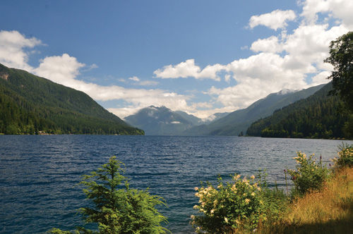
FIGURE 26-1 This is Crescent Lake in the Olympic National Park in Washington state. Every organism in the scene—plus all those in the Olympic Peninsula—are part of a community. At the same time, organisms in the lake interact more with each other than they do with the conifers, and the lake is also a community within the larger community.
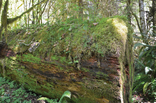
FIGURE 26-2 The organisms on this fallen log constitute a smaller community than all the Olympic Peninsula, not only in space but in time. This area—the log—did not exist as a habitat until the tree died and fell; after that it could be occupied by fungi, bacteria, mosses, ferns, and even tree seedlings. But this community will last only 100 years or less, until the log decays away.
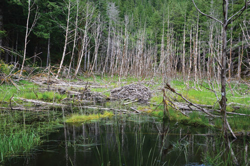
FIGURE 26-3 The pile of branches is a beaver house; the water around it is a pond created when a beaver built a dam across a small stream. The dam has already changed the habitat and community: The dead standing trees were killed when the rising water of the pond drowned their roots.
Communities also have boundaries in time: They come into being and then cease to exist. In the American west, beavers build dams across narrow rapidly flowing streams, converting them into broad shallow lakes with water that flows slowly (FIGURE 26-3). A pond comes into existence, and its characters differ from those of the stream. The first change is that a beaver family lives in it and fertilizes it with their urine and feces. The shallow, quiet waters at the edge of the pond allow certain plants to grow that could not tolerate the stream’s rapid flow; as the pond fills, it floods and drowns nearby trees, thus allowing more light to penetrate when the trees die. Fish, turtles, and other animals respond differently to ponds than they do to streams, so the pond community quickly becomes different from the stream community that had existed before. A beaver pond community typically changes with age as more plants invade its edges and trap silt, gradually turning the margins of the pond into land. Later the entire pond usually becomes a broad, flat meadow and the pond community goes out of existence (FIGURE 26-4). Many factors such as fires, volcanic eruptions, erosion, hurricanes, and other disturbances alter patches of territory and in the process destroy some communities but permitting new ones to start.
Even if climate and geology remain the same throughout the lifetime of a community, some communities change as part of their very nature whereas others remain the same. A beaver pond automatically changes with time because the life activities of the first organisms to colonize the new pond—the pioneers—change the pond such that it is better suited to other organisms than themselves. Each new group of organisms alters their habitat such that they themselves are excluded and new species come in. This more-or-less predictable sequence of changes is called succession and it occurs in many communities.
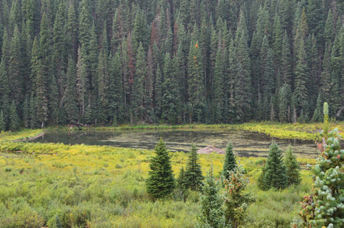
FIGURE 26-4 This is a much older beaver pond, gradually changing into a meadow. The land surrounding the open water is flat—flat land does not occur in mountainous areas like this except through the silting in of a pond, usually a beaver pond. Already, marsh plants are growing over most of the flat area; soon tree seedlings will be able to survive there as well. The beaver family will have to find a new stream.
In contrast, some communities remain the same for many years. Spruce-fir forests cover thousands of square kilometers and endure for thousands of years. In this situation, the various members of the community alter the habitat so that it remains beneficial for themselves and is not suitable for other species that might try to invade. Even if there is a major disturbance, such as a fire or landslide, the pioneers that come in after the disturbance, such as quaking aspen (Populus tremuloides), alter the area such that it becomes suitable for spruce-fir forest again. The disturbed patch undergoes succession until it becomes spruce-fir forest again, which is the climax community, and stability returns (FIGURE 26-5).
These examples illustrate an important concept. Most communities are patchworks of coexisting species, and they are all maintained by various processes. The processes are those described in Chapter 25, such as disturbance, competition, predation, mutualism, commensalism, and so on. In community ecology, we attempt to analyze these for several members of the community to try to understand how these processes result in the various patterns that we call communities.
Community ecology is important to us because we are members of every community in which any human lives, works, plays, or goes to reconnect with nature. As members of so many communities, we affect the other organisms, and we would like to know what impact we are having. Throughout much of history, we have tried to conquer nature or at least tame it: We exterminated the passenger pigeon completely, killing every single member of the species and driving it to extinction. We did our best to purposefully exterminate wolves, bears, bison, and prairie dogs. Each is an example of selectively removing one important species from communities. We need to know how various communities respond when key organisms are eliminated. We damned rivers for power, navigation, irrigation, and flood control. And in so doing we altered the physical aspects of many communities, flooding some out of existence, altering the natural cycle of springtime floods and summers with low water. Dams also prevent fish from migrating upstream for spawning, and have greatly reduced salmon runs.
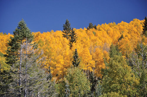
FIGURE 26-5 This patch of quaking aspen is growing in an area of spruce-fir forest that was burned in a forest fire. Quaking aspen seedlings must have bright light; they don’t survive in a patch of spruce and fir forest where the ground is heavily shaded. But after a fire, quaking aspen seeds are blown in, germinate, and grow vigorously. Seedlings of spruce and fir also germinate, but cannot grow nearly as rapidly as those of quaking aspen, so they suffer. But quaking aspen trees are short-lived and die quickly, gradually making way for the spruce and fir seedlings; this patch will gradually revert to spruce-fir forest.
Fortunately, the attitudes of many people have changed to one of striving to live with nature as harmoniously as possible, to have minimal impact on other organisms. We have begun various projects in community restoration, such as reintroducing wolves into Yellowstone National Park and encouraging the migration of bears and mountain lions across the Rio Grande River from Mexico into Big Bend National Park in Texas. Several dams have been removed, most notably the Elwha and Glines Canyon Dams on the Elwha River in the Olympic National Park in Washington state, to restore the rivers so that fish can complete their life cycles (FIGURE 26-6). Very ambitious efforts are underway to reestablish tallgrass prairie communities that were part of the grassland ecosystem that covered all the Plains States until it was destroyed for wheat farming during World War I. Fortunately, at least a few individuals of most species still exist scattered throughout the area, many of the plants surviving as weeds along railroad rights of way. These projects go beyond restoring a community; we need to completely rebuild it, but we are not certain of the proper methods. Just bringing all plants and animals together at one time and place has not been successful. It may be that we will need to introduce certain pioneer species and then later add others, in effect trying to mimic or encourage succession; this may be more effective than trying to assemble a climax community all at once.
Even though we are trying to live more harmoniously with nature, we still need to farm, build towns, mine for minerals, and so on. This inevitably leads to habitat loss and habitat fragmentation, but by studying community ecology, we may be able to minimize the damage we do. We already realize that wetlands are extremely valuable; not only do they have high species diversity, but they also filter harmful chemicals out of water, prevent erosion, and produce abundant animal life. Most cities and states now protect wetlands and direct construction projects into areas that are not as sensitive. Similarly, as we set aside land for parks and wildlife preserves, planners need information about the dynamics of the communities involved: If a population of animals is to be protected, we must set aside enough habitat—and the correct habitat—that will allow the animal to find food, mates for reproduction, and protection from predators. Rather than one large preserve, it may be better to set aside multiple smaller ones interconnected by protected corridors such that animals can migrate from one to another freely (FIGURES 26-7A and B).

FIGURE 26-6 Removing this dam will allow the stream to flow naturally again. Spring floods will redistribute sand and sediment, low flows in summer will allow streamside communities to flourish. Fish will be able to migrate and other organisms will once again have suitable habitats that had been destroyed when the dam was constructed.
We human beings, Homo sapiens, are the most destructive species to have ever evolved, but fortunately we are also the most intelligent. A large percentage of us recognize the damage we have done and are still doing, and many of us are working hard to find ways to live more responsibly. Research into community ecology will give us the knowledge and tools we need to do the most good as quickly as possible.
![]() Diversity
Diversity
Communities consist of more than one species, but how many more? Some communities, such as salt flats or sand dunes, have only a few species whereas others, such as rain forests, have thousands. Some are obviously more diverse than others, but that is often easier to see than to measure. A first approach to quantifying community diversity is done by measuring species richness, which is simply a count of the species present. This count is a species checklist, and all national parks and wildlife preserves have checklists available. But checklists are always incomplete because it is impossible, and usually not necessary, to catalog every prokaryote and fungus species present. And for organisms such as invertebrates, mosses, and even ferns, there are not enough trained specialists available to catalog all such organisms present in many areas. Studies of community ecology focus only on several organisms rather than all of them, so it is not necessary to have a complete checklist.

FIGURE 26-7 (A) This overpass is a short migration corridor; it is covered in grass and herbs and is intended to provide a safe passage for deer and other animals across the highway. It is located in the Flathead Indian Reservation in Montana. (B) Corridors that provide a safe route for animal and plant migration are usually many kilometers long and interconnect two or more wildlife preserves. Often, they follow river valleys, as depicted here.
Factors other than species may be the objective of studies of diversity. Instead, diversity of growth forms may be the focus, such as the presence, absence, and relative abundance of herbs, shrubs, and trees, or of annuals, perennials, and ephemerals (FIGURES 26-8 and 26-9). When studying the feeding methods of herbivores, it might be important to understand the diversity of plant storage organs, whether they are present below ground as bulbs, taproots, and rhizomes or instead are located above ground as fruits, seeds, and edible shoots. Other studies might examine the diversity of primary producers, primary consumers, secondary consumers, decomposers, and so on, and how they interact with each other. At present, DNA technology allows us to even study the diversity of alleles present within a community. It might be tempting to ask “Which is the real diversity?” They all are real; they all contribute to the richness of life in even small areas. It is never possible to study everything simultaneously, so we must define our hypotheses then formulate questions that are simple enough to be tested.
FIGURE 26-8 Coastal marshes, such as this Sabine National Wildlife Refuge in Louisiana, have many species of both plants and animals but a low diversity of growth forms. Almost all plants are herbs with foliage that dies back in winter and then regrows in spring. Many are rhizomatous, but there are no trees or shrubs, no succulents or epiphytes, and only an occasional vine.
FIGURE 26-9 The temperate rainforest in the Olympic National Park has an extremely high diversity of both species and growth forms. Numerous species of conifers are present and dominant, but there are also deciduous angiosperm trees and bushes, ferns, mosses and liverworts, many plants with bulbs or rhizomes, and a large diversity of epiphytes and vines.
Diversity and Scale
Whichever aspect of community diversity we might be studying, a common observation is that scale matters. Larger areas are more diverse than smaller ones (FIGURE 26-10). For example, if we consider the entire Earth to be our community, it contains every species, every growth form, and so on, whereas a smaller area—the Americas for example—might still have as many growth forms, but would not have as many species. Similarly, a plot of land, perhaps one planned as a wildlife preserve, 100 km × 100 km will almost certainly be more diverse than an area only 1 km × 1 km. Finding higher diversity in larger areas is common; often the underlying causes are easy to understand. A larger area will have more variation in types of soil, topography, geology, and so on. It has more diverse habitats so it can have more types of organisms, each adapted to particular aspects of the area. Second, larger areas have larger populations than does any smaller sub-region of that area. During a disturbance such as a drought or fire, larger populations are less likely to die out than smaller ones. We are not talking about a species going extinct, just simply that if there are only a few plants or animals in an area, they might all die at some point, temporarily diminishing the diversity of the area, but a year or two later they might reappear as new seeds are carried in or as animals travel from one region to another.
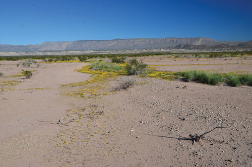
FIGURE 26-10 The importance of scale when measuring diversity is immediately obvious in this area of Big Bend National Park in Texas. The area here is rich in short-lived yellow flowers (Baileya multiradiata). If this area were divided into sample plots 1 m2, some would have no plants at all, others would have a few yellow flowers, and other plots would have yellow flowers, creosote bushes, grasses and several shrubs. Diversity in this outwash area varies with distance from the small, temporary stream. The entire park is extremely heterogeneous on a scale of kilometers: The east side is rich in cacti, agaves and yuccas; the west side has sotols and ocotillos; the Rio Grande river has water plants; and the Chisos Mountains have a subalpine flora.
The relationship between area and species richness is called the species-area relationship and is expressed by the formula
S = cAz
in which S is the number of species, A is the area, and c and z are constants that must be discovered by studying individual communities. Once c and z are known for various communities, they can be used to compare the diversity of those communities.
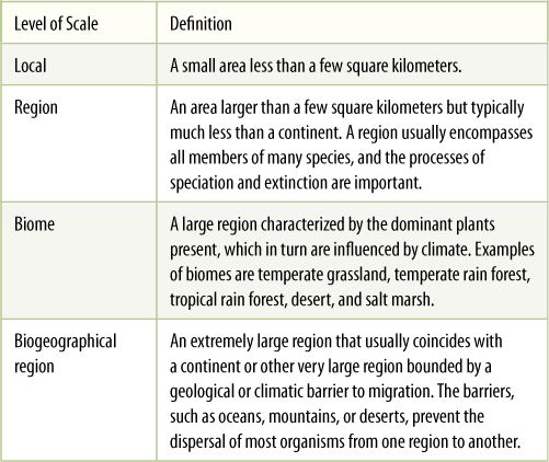
Because scale is so important in community ecology, several distinct sizes are typically used, as shown in TABLE 26-1. Most studies are carried out in research areas that fall into the “local” designation. Based on the regions of Table 26-1, Robert Whittaker proposed a means of measuring diversity at specific scales:
1. Alpha diversity is the number of species or growth forms that occur at a local, small site.
2. Beta diversity compares differences between several small sites within a larger region. The region should be the larger community being studied; the comparison is between various plots within a forest, for example, not between some in a forest and others in an unrelated desert.
3. Gamma diversity is the number of species within a region.
TABLE 26-1 Various Level of Spatial Scale
In all such research, determining the size of the area to be studied is problematic; often preliminary studies must be done to be certain that an expensive long-term study will not be wasted by focusing on plots that are either too small or too large.
No community will have equal numbers of individuals of every species. Instead, several species have an abundance of individuals and are common whereas most species have just a few individuals and are rare. Checklists and species-area relationships do not reflect this; instead they treat all species equally. As an alternative, we can plot the number of species in each abundance class and obtain a species abundance distribution. One theoretical distribution is that shown in FIGURE 26-11, in which most species in an area are very rare; a survey of a sample area would find several species dominating the area (right side of the graph), but most species would be rare, and a researcher would have to hunt carefully to find the one or two individuals of most species. This is a common experience in both fieldwork and casual hikes: One notices hundreds of plants of the most common species, several plants of a rare species, and will be lucky to find even a single plant of the least abundant species. Chances are good that we might not find even a single specimen of the rarest species unless we hike the area many times, or take alternative routes, all the time seeing so many plants of the most abundant species that we no longer pay any attention to them.
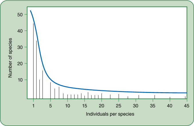
FIGURE 26-11 In this theoretical model of species abundance distribution, most of the species have only one or two individuals in the sample (extreme left side of graph). In contrast, only a few species have as many as 5, 10,… 25 individuals in the sample (only one or two species in each abundance class in the center of the chart). On the right, one species has 36 individuals in the sample, another has 44; these two species dominate the community.
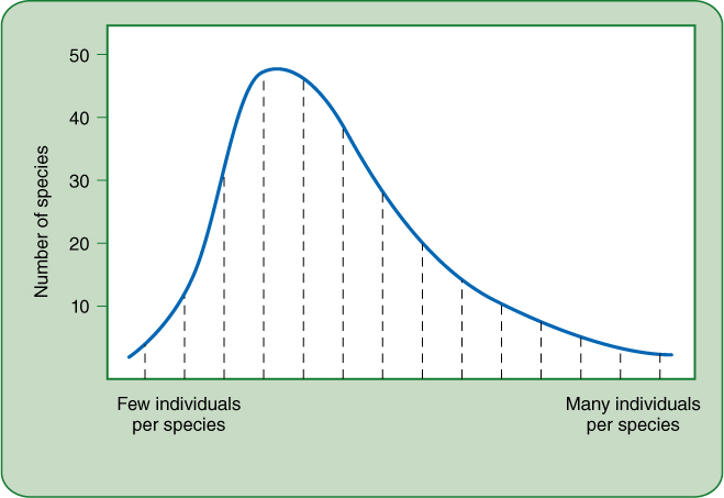
FIGURE 26-12 This theoretical model of species abundance distribution is more realistic than the one in Figure 26-11. Here too the sample is dominated by a few species with many individuals (right side of chart), but on the left side, the line is very low, indicating there are only a few species that are truly rare. Most species (center of the chart) have a low population density but are not rare.
But research has shown that species abundance distributions such as that shown in Figure 26-11 do not describe most communities accurately. A community might have a few species with only one or two individuals, but that would not be true of most species. Most species might be rare, but not that rare. If a distribution similar to that in Figure 26-11 is found by research, then the problem is almost certainly that the sample areas were too small or had not been search carefully enough. Communities that are sampled extensively and accurately usually have a species abundance distribution similar to that in FIGURE 26-12: There is a peak (a mode) of species with a sparse number of individuals, a few that are truly rare (to the left of the mode), and a few that are very common (to the extreme right of the mode). Most communities are dominated by a few abundant species but most species are sparse, and several species are rare.
Diversity and Latitude
Diversity varies with scale, as just discussed, and it also varies with latitude. Even early naturalists noticed that far northern areas in Canada, Siberia, and Alaska have far fewer species (lower diversity) then do similarly sized areas near the equator in the Amazon rain forest, central Africa, and Southeast Asia (FIGURES 26-13 and 26-14). Many theories about the causes of this latitudinal diversity gradient have been proposed, and exploring several of these ideas will give us insight into the complexity of the patterns and processes of community ecology.
Perhaps one of the oldest and still most widely taught theories is that the tropical regions near the equator have relatively benign environments whereas those at higher latitudes have more severe conditions. Near the equator, temperatures are always warm; freezing conditions are extremely rare except on the highest mountains. Rainfall is abundant with only occasional short periods of dryness. Plants do not have to be adapted to survive freezing or water stress. In contrast, the only parts of Antarctica, Greenland, and Iceland that are not permanently covered by ice sheets are small areas along their coasts. Alaska, Canada, Scandinavia, and Siberia are so far north they receive little sunlight or warmth throughout winter, and temperatures are bitterly cold. During summer, only the uppermost few centimeters of soil thaw, so vast regions are underlain by permafrost, a permanent layer of ice that does not allow roots to penetrate or water to drain away. The summer growing season at high latitudes is brief and cool; the sun is low in the sky so very little energy is available to the plants—the primary producers—so there is very little energy available to any other component of high latitude communities. Few organisms can adapt to such harsh conditions, so high latitudes have lower diversity than do equatorial latitudes.
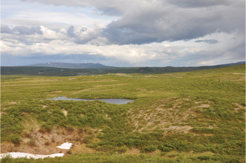
FIGURE 26-13 Community diversity is very low in the high latitudes of northern Alaska. This tundra is dominated by just a few species of low bushes and some perennial herbs. Snow is present even though this is June, and most subsurface soil is frozen.
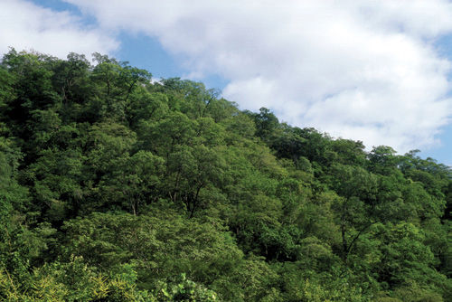
FIGURE 26-14 A tropical rainforest, such as this area of Bolivia, has high diversity of both species and growth forms. Only trees are obvious in this image, but there are many species of trees in this one image, and a closer view would show epiphytes, vines, parasitic plants, bulbs, and many others. Rocky outcrops will typically have cacti and drought-adapted plants even in the midst of a rain forest.
This ecological explanation is satisfying but it is not the entire explanation. Geographical and geological components also contribute to the differences in diversity. There is definitely low diversity of plant species in the high latitudes of the southern hemisphere, but mostly that is due to the fact that there is almost no ice-free land there. Antarctica is the largest land mass, but it is covered in ice except for a few square kilometers along the coast, an area in which only two species of angiosperms survive (a grass, Deschampsia antarctica, and a species of the carnation family, Colobanthus quitensis); this is the lowest diversity of flowering plants known. Much of the rest of the temperate southern hemisphere is ocean, with the only habitable land being Australia and New Zealand plus the southern tips of South America and Africa. The temperate latitudes of the northern hemisphere have more land, but much of that too is either covered by ice or consists of mountain ranges whose peaks are frozen. Alaska and western Canada are mountainous, as are Scandinavia and eastern Siberia (FIGURE 26-15). In contrast, the region between the Tropic of Cancer and the Tropic of Capricorn contains extensive land masses consisting of almost all the land of Africa, Southeast Asia, and the Americas from Mexico to the south of Brazil and Peru. This area contains some mountain ranges, but few are so tall as to have their peaks permanently covered in ice. Instead there are the enormous lowland plains of the Amazon, central Africa, and much of India and Southeast Asia. Tropical regions simply have more land available for plants—primary producers—and thus more land for all sorts of organisms.

FIGURE 26-15 Much of the far northern latitudes are mountains with permanent snow cover, areas where plants cannot grow. Even though there is abundant land, it is unavailable for most living organisms. These are the Chugach Mountains near Anchorage, Alaska.
We are just now obtaining new types of evidence that indicates that evolutionary history is also a fundamental contributor to the differences and diversity between tropical and high latitude areas. Until 50 million years ago (mya), Earth’s climate was much warmer than it is now (FIGURE 26-16), and tropical conditions covered almost all of Earth’s land masses. The Rocky Mountains, Andes Mountains, and Himalayas had not yet formed, so there were few snow-covered peaks. Antarctica was farther north and not yet frozen over. With the warmer temperatures, oceans evaporated more water, which was carried by air until it fell as rain, so most of Earth’s land had a warm, moist, tropical climate. Fifty million years ago, ferns and conifers were diverse; angiosperms too had originated and diversified but many of the most modern groups had not yet come into existence.
At 50 million years ago, Earth’s climate began to cool, temperatures began to drop. At 40 mya global temperatures were so cool that the Antarctic ice sheet had begun to form. Mountain peaks had snow more frequently and for longer periods each year, then many became permanently snow-capped; the plants that had been there died by being buried in snow. Glaciers formed in mountains and then at about 12 mya, ice sheets began to cover Canada, Europe, and Russia; any plants in the region were scraped away by moving ice. Because the oceans too became colder, less water evaporated and less rain fell on land. Cool, dry, temperate conditions spread across Earth; the huge area of the United States and Russia were still warmer and more humid than today, but they were changing from tropical to temperate. Tropical climate contracted to encompass just the equatorial region.
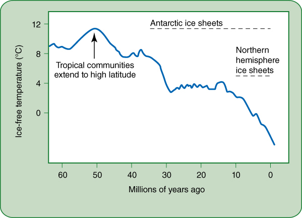
FIGURE 26-16 The average temperature of Earth was much higher until about 50 million years ago, then began dropping more or less steadily. By 40 million years ago, permanent ice sheets began to form on Antarctica; 10 million years ago, glaciers pushed out of mountains in the northern hemisphere, and some in the far north coalesced into gigantic sheets that moved across all of Canada and the northern United States, while others covered Europe and Siberia.
This new knowledge of Earth’s climate history indicates that temperate conditions are recent. Whereas plants and animals have had hundreds of millions of years to evolve and adapt to tropical conditions, they have had only a few tens of millions of years to adapt to temperate conditions. This hypothesis predicts that many genera or even families of temperate flowering plants should have evolved from ancestors that were adapted to tropical conditions. Current research into angiosperm phylogeny is consistent with that: Many clades of temperate plants are nested within tropical clades; they do have tropical ancestors. This means that one of the causes of the high diversity of tropical regions is simply that there has been much more time for organisms to become adapted to those conditions and to each other, more time for niche partitioning and coevolution. In contrast, there has been less time to adapt to temperate conditions, and such adaptations may have been difficult. Plants that evolve from being tropic-adapted to temperate-adapted need to have structures and physiologies that are unnecessary for tropical plants. Temperate-adapted plants need to use day length to detect autumn and prepare for winter. Leaves must be abscised or winterized. Well-protected resting buds are needed, and even the vascular cambium must become dormant in winter, capable of resisting very low temperatures. Ring-porous wood with strongly differentiated earlywood and latewood is advantageous, as are storage organs like bulbs and tubers, and large parenchymatous rays in wood and bark. Obviously natural selection did produce adaptations necessary for survival in temperate conditions, but there really has not been much time to refine the adaptations or to allow them to diversify. If temperate regions would remain temperate for several hundred million years longer, then perhaps species diversity in temperate latitudes eventually would become as high as it is in tropical ones.
![]() Predator—Prey Interactions
Predator—Prey Interactions
One Predator, One Prey
To understand predator—prey interactions, we will begin with the simplest system, in which one species of prey, such as a plant (a primary producer), is attacked by only one species of predator, such as an herbivore (a primary consumer). Within natural communities, any plant is attacked by multiple predators, and almost every herbivore attacks several species of plants. But the one predator—one prey model is useful because it helps us understand how we human predators should harvest our various prey, such as fish, deer, lumber, and so on (FIGURE 26-17).
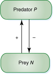
FIGURE 26-17 In this simple diagram of one species of predator (P) consuming one species of prey (N), the positive arrow indicates that the presence of the prey species benefits the predator species, whereas the negative arrow indicates that the predator is harming the prey.
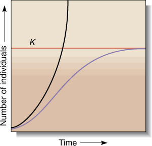
FIGURE 26-18 The line labeled K represents carrying capacity. Instead of increasing infinitely (black curve), the growth rate (purple curve) decreases as the population size approaches the carrying capacity of the habitat. When population size equals carrying capacity, population increase stops; the death rate equals the birth (germination) rate.
Assume that the prey population grows logistically, as shown by the purple line in FIGURE 26-18. On the left side of the graph, population density is low, every plant has space, light, and water, and most seeds germinate. There are unused resources, so if more plants were present, the population growth would be faster. On the right side of the graph, population density is higher, plants compete for resources, not all seeds find a suitable space for growth; if more plants were present, there would be more competition and population growth would slow. On the extreme right side, the community is supporting as many individuals of the species as it can: The population has reached its carrying capacity K.
Now assume there is a species of predator—some type of herbivore—that feeds exclusively on the plant. The predator’s population density will grow logistically as shown in Figure 25-23B, and for our purposes, the factor that controls its population increase is the amount of prey available. The population densities of these two interacting species may follow one of three paths. First, as the herbivore consumes more of the plant, the plant population decreases, which in turn makes it more difficult for the predator to find food, so its population decreases also. The two populations may cycle up and down repeatedly (FIGURE 26-19). Second, the predator may consume so much of the prey that the prey population becomes low or even locally extinct, which in turn may cause the predator to become locally extinct also. Such a predator—prey pair would not be part of a community for long. Third, other factors may limit the population of the predator such that it cannot overconsume the prey and both species remain at low, stable population sizes indefinitely.
Two fundamental aspects of predator—prey relationships are the predator’s feeding rate and its handling time. Feeding rate refers to how quickly a predator find a new prey individual, and handling time refers to the amount of time needed to actually consume the prey. The two together constitute the predator’s functional response. Feeding rate will be faster if there are more prey individuals available, so a predator’s functional response is dependent on prey density, it is prey-dependent.
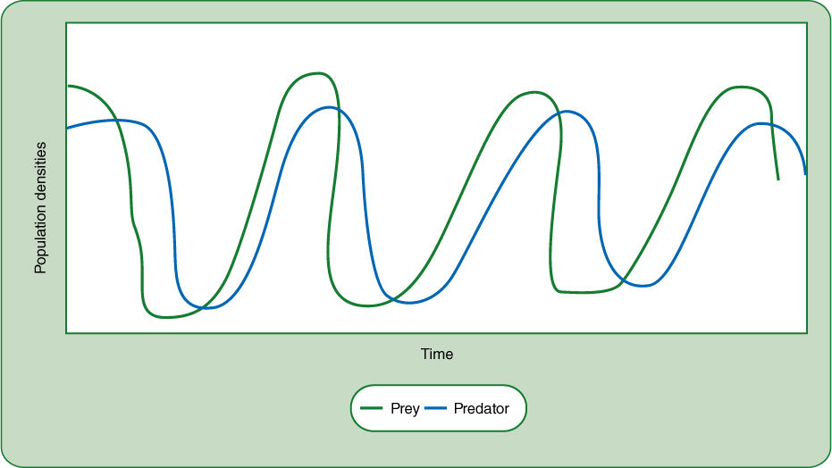
FIGURE 26-19 This graph is one theoretical possibility for cycling of predator and prey populations. As the prey population grows, so does the predator population, but at some point the predator consumes too much of the prey, whose population then declines. This leads to a decline in the predator population, and the rise and fall of predator numbers always lags somewhat behind prey numbers. This model shows the populations falling to very low densities, but that is not necessary for many species; a moderately sparse population of prey would be enough to cause predator numbers to fall. Also, this model assumes that the each individual predator consumes many prey, such as one deer grazing many grass plants. But sometimes predators are smaller than prey; if this were showing ticks attacking deer, or aphids attacking plants, the predator populations would be much larger than those of the prey.
The simplest model of single predator—single prey interaction is the Lotka-Volterra model. It models the net rate of change in prey numbers as
dN/dt = rN — aNP
in which dN/dt is the rate of change with time of the prey population
r is the intrinsic rate of increase for the prey species
N is the number of individuals of prey species in the community
a is the predator’s per capita attack rate
P is the number of predator individuals present.
The units of a are the number of prey eaten per prey per predator per unit time. That is, a is also prey-dependent; it is small if few prey are present, larger if prey are abundant.
The equation for the net rate of change of predator numbers is
dP/dt = faNP — qP
in which dP/dt is the rate of change with time of the predator population
f is a constant indicating the predator’s efficiency at converting the prey it has eaten into new predators
q is the predator’s per capita mortality rate (which is independent of population density).
The population of prey will be stable, neither increasing nor decreasing, when dN/dt = 0, which can be expressed as
rN — aNP = 0
rN = aNP
r = aP
r/a = P.
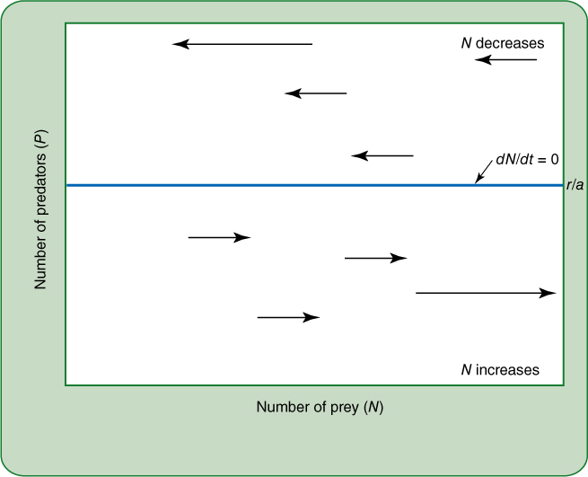
FIGURE 26-20 The zero growth isocline for prey, as modeled by the Lotka-Volterra hypothesis. Just consider the vertical axis on the left, the number of predators. At any point below the zero growth isocline, the number of predators is too low to prevent the prey population from growing. For example, if there are just a few deer, grasses will still flourish and increase in abundance if they have not yet filled the habitat as fully as possible (if they have not reached the carrying capacity, K). But if the predator population is at any level above the zero growth isocline, there will be so many predators that the prey population will decrease. If the predator population is exactly the density of the zero growth isocline, then the prey population will neither increase nor decrease: There will be zero growth.
The prey population is stable when the density of the predator equals r/a. Similarly, the population of predators is stable when dP/dt = 0, which can be expressed as
faNP — qP = 0
faNP = qP
N = q/fa.
That is, the predator population will be stable when the density of prey equals q/fa. Notice that for both predator and prey, stable conditions are defined by r, a, q, and f, all of which are constants. Thus they can be represented on graphs as straight lines. In FIGURE 26-20, the line dN/dt = 0 indicates the predator population that will keep the prey population stable. If the predator population is sparser than that of the line, the prey population will increase; if predator populations are greater than the line, the prey population decreases. The line indicating population stability is called a zero growth isocline. FIGURE 26-21 illustrates the effect of prey density on predator populations. Both are easy to understand without the equations, but an important relationship is revealed when the zero growth isoclines of both predator and prey are placed on the same graph as in FIGURE 26-22. The point at which the two zero growth isoclines intersect indicates the population sizes of predators and prey that can coexist stably. If some factor causes one population to change, that factor will also affect the other population. Starting in the lower left quadrant, with both predator and prey populations low, an increase in prey populations will cause the predator population to increase. In the lower right quadrant, high prey populations cause the predator population to increase so much that prey numbers begin to decrease. The two populations cycle as indicated by the arrows. This is another method of representing the concept of predator—prey cycling as illustrated in Figure 26-19.
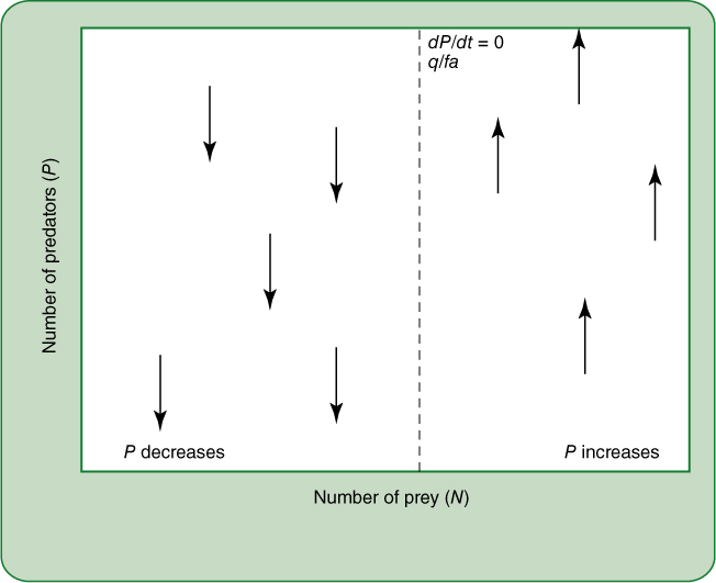
FIGURE 26-21 The zero growth isocline for predators, as modeled by the Lotka-Volterra hypothesis. This is similar to Figure 26-20, except that here we are considering the effect of prey populations on the predator density. Any population of prey that is too low (that is, to the left of the zero growth isocline) will cause the predator population to decrease; any population of prey to the right of the isocline will cause the predator population to increase.
The Lotka-Volterra model has been criticized for being too simplistic and at present its main value is its ability to simplify complex interactions while teaching the fundamentals of predator—prey relationships. Another model, the Rosenzeig-MacArthur model, adds more factors that affect both predators and prey in real communities. Its equations are only slightly more complex than those presented here, but the important point for us is that in this more realistic model, the zero growth isoclines are curves rather than straight lines, and relationships between stable and unstable populations are more complicated. FIGURE 26-23 illustrates a curved zero growth isocline for a prey species. If a predator is rather inefficient at consuming its prey, the prey population will be mostly controlled by other factors. The zero growth isocline for the predator will be to the right of the hump (Figure 26-23) and this will be a stable relationship. If the predator is very efficient at consuming prey and keeps the prey population low, the two zero growth isoclines will intersect to the left of the hump and this will be an unstable situation (FIGURE 26-24). The predator at some point may overconsume the prey and cause both to be eliminated from the community.
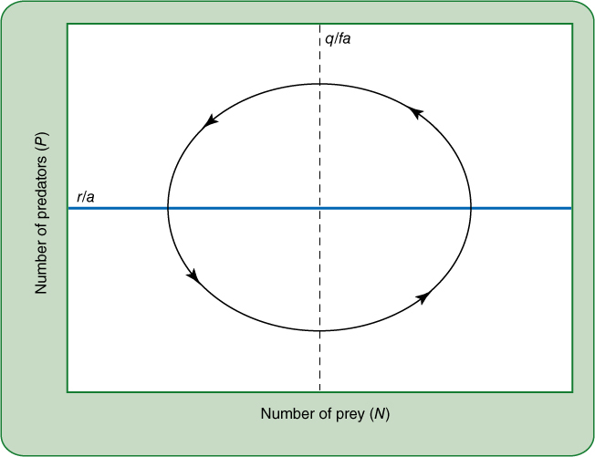
FIGURE 26-22 The only point at which both predator and prey populations will remain steady, neither growing nor decreasing, and not even cycling as in Figure 26-19, is the point where the two zero growth isoclines intersect in the middle of the graph. But such steady conditions are extremely unlikely, and any number of factors other than the presence of the other species can cause either the predator or the prey to decrease or increase. If this happens, then the change of one species of the predator—prey pair will cause the other to respond, and in this case, the response causes a continual cycling of both populations.
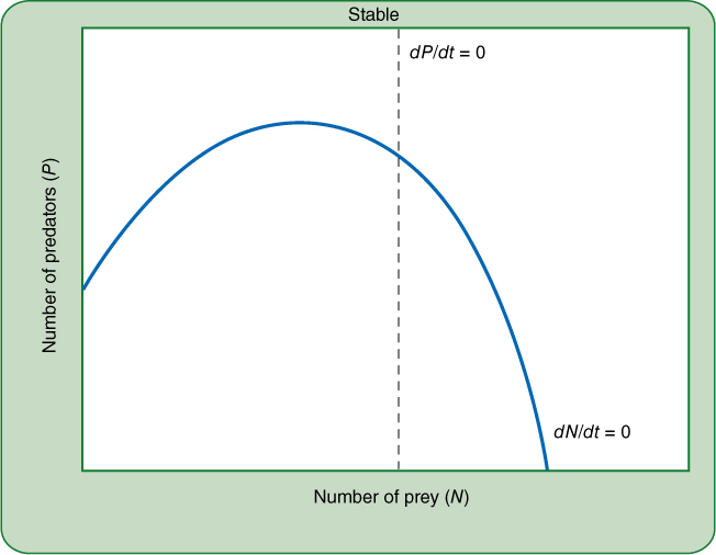
FIGURE 26-23 This curved zero growth isocline for the prey species is more realistic than the straight line in Figures 26-20 to 26-22. If the zero growth isocline for the predator intersects it to the right of its maximum, a stable situation results: Any disturbance tends to bring the two species back into equilibrium. Keep in mind that these are just two hypothetical species; in real life, we would need to study particular predator—prey pairs in particular communities to see what the zero growth isoclines are and where they intersect. Simply changing the habitat could alter both of these lines for the two species we are considering.
The curved zero growth isocline has unexpected consequences. Imagine a stable situation as in Figure 26-23 with prey populations high due to an inefficient predator. Changing conditions might increase the habitat’s carrying capacity for the prey; for example, more rain or warmer temperatures or more nutrients might cause the habitat to support a higher density of the plant species. It seems as if this should also benefit the predator—there will be more prey to eat—but that is not always true. As conditions for the prey improve, its zero growth isocline will rise and the hump may shift to the right enough that the intersection between the zero growth isocline is now to the left of the hump (FIGURE 26-25) and the predator—prey interaction becomes unstable. Improving conditions for the prey may lead the predator to overexploit the prey and both species will be lost. This is called the paradox of enrichment and may be an important factor in the loss of species diversity when a habitat is “improved.” An example would be eutrophication, in which mineral-rich pollution fertilizes streams and lakes, causing certain algae to proliferate but ultimately resulting in loss of many species (see BOX 12-1).
We harvest many wild species from the environment, so we have a predator—prey relationship with those organisms. We have the ability to choose whether we will harvest moderately such that our prey (fish, lumber, deer) can remain at high, stable populations. For organisms that have a sigmoidal growth curve (Figure 26-18), the population’s maximum per capita productivity is the inflection point at which growth rate changes from positive to negative. Theoretically, if we would harvest just enough of a species to keep the population density at that point, the species would be stable and we would obtain what is called a maximum sustained yield. However, we do not know enough about the growth characteristics or population sizes of most species to determine that point, and if we err by harvesting too much, we put the species in danger. This has occurred with many species of fish, whales, turtles, and other marine life that have been overharvested to the point at which many are rare and must now be protected.
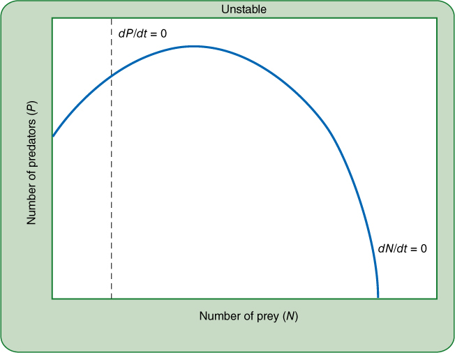
FIGURE 26-24 If the zero growth isoclines of predator and prey intersect to the left of the prey’s maximum, the situation will be unstable. A disturbance may cause the two populations to cycle, but there is a strong possibility that the predator will at some point overconsume the prey and populations of both will drop and not recover.
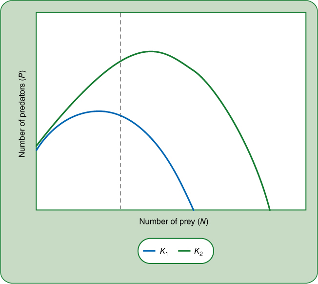
FIGURE 26-25 The paradox of enrichment. Improving the environment for one of the two members of a predator—prey pair may result in loss of both species. In the case illustrated here, improving the habitat such that prey grow better causes their zero point isocline to increase and its maximum to shift to the right. The intersection with the predator’s zero growth isocline has changed from a stable point to an unstable one: If the habitat becomes more favorable for the prey, that may lead to its initial increase which causes an increase in the predator and may result in enough overconsumption that the prey is eliminated from its improved habitat.
An alternative is fixed effort harvesting in which population health is determined by the amount of fish or deer, etc., that can be harvested with a particular amount of effort. If populations are healthy, the harvest will be abundant; if populations are sparse, the harvest will be poor, but either way, harvesting must be stopped after a particular amount of effort or time. For example, hunting or fishing is allowed only for a fixed length of time. Theoretically either harvest will not damage the population too severely because we automatically harvest only a few individuals if the population is sparse but harvest many when the population is healthy. A common alternative is fixed quota harvesting in which fisherman or hunters are allowed to harvest a particular amount, such as one deer per hunter or a certain number of tons of fish per fleet, no matter how long it takes or how much effort is required (FIGURE 26-26). Obviously, if populations are low and threatened, hunting them until a particular quota is reached will cause great harm. Unfortunately, both methods rely on governments to set the quota or the effort level, and governments often yield to pressure from industry or sportsmen to increase the legal harvest despite the risk of harming the species.
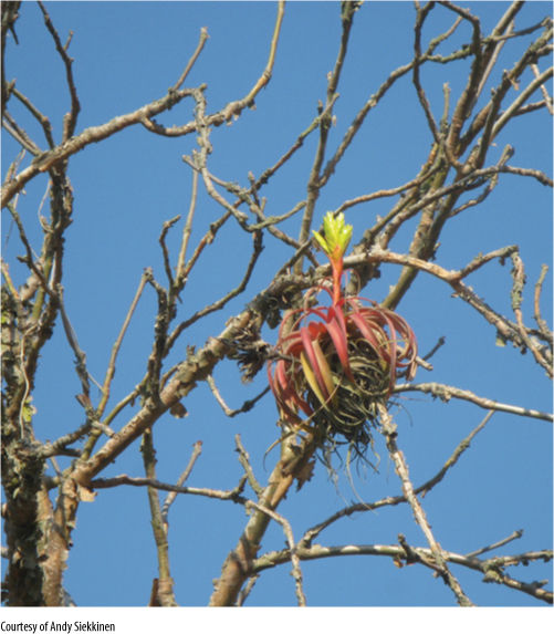
FIGURE 26-26 Many exotic plants such as orchids, peperomias, cacti, and bromeliads such as this Tillandsia rothii are still collected from the wild. For some species, the numbers of plants collected each year is so low that collection does not significantly affect population numbers. But others are so popular and have been collected in such high numbers that collection was a significant threat and now all collection of many species is banned: There is a fixed quota of zero.
Plants Do Things Differently
BOX 26-1 Plants and Animals Are Different Kinds of Prey
In many models of predator—prey interactions, both the predator and the prey are considered to be animals: One animal eats another animal. But because plants are the primary producers in terrestrial communities, most of the prey biomass and the greatest number of prey individuals are plants. Why do models and equations focus more on animals rather than plants?
Plants and animals respond differently as prey. Animals can fight back, flee, and hide, whereas plants can only remain rooted to the ground, perhaps protected by spines or poisons. But more importantly, when a prey animal is attacked, it is usually killed and eaten. The consumer may eat all the prey animal or may leave some for scavengers, but either way, the prey animal is dead and gone: The number of prey individuals decreases by one. Even if the prey animal somehow survives an initial attack with only a wound, that will probably weaken it to the point that it will be killed and eaten in the next day or two.
But plants do things differently, and it is difficult to kill a plant. If you spent time gardening with your parents, you have heard “Be sure to pull out the root.” Few plants are killed by ripping off some leaves or branches; even breaking off the shoot and leaving the root in the soil will not kill a plant if, at the top of the root, there is a bit of stem with an axillary bud that can produce a new shoot. Caterpillars routinely eat every leaf off a tree (they defoliate the tree) without really harming the tree; many trees survive being completely defoliated twice in the same year. Deer browse off young twigs and leaves, cattle and bison graze all the leaves off grasses, but none of this ever kills the plant. If we count only the numbers of individuals, thousands of herbivorous consumers can prey on a patch of plants for years without the loss of even a single plant. This is very different from one bobcat killing hundreds of rodents during the same time.
To handle plants as prey, it is usually necessary to have models and equations based on kilograms of biomass instead of numbers of individuals. In some cases, it is relatively easy to measure the amount of plant biomass lost during predation: A control patch can be mowed to collect leaves, which are then weighed and compared to the experimental patches. But it is more difficult to measure the weight or amount of leaves and twigs lost from bushes and trees, or the number or weight of small seeds lost to granivores. In addition, most plants are attacked by multiple predators, many of which are easily overlooked—aphids, fungi, and nematodes, to name just a few. It is difficult to measure the effects of grazing if we cannot quantify the harmful effects of other organisms that are simultaneously attacking the plant.
Especially harmful with marine life, every nation sets its own quotas, and even now both Norway and Japan allow harvesting of various species of whales even though they are endangered. In this case, anyone is allowed to hunt or harvest in the “common area,” that is, the parts of the ocean that are not claimed by any nation. The ocean floor and all of Antarctica are also considered common areas. For each country, it is to its own advantage to harvest as much as possible before some other country harvests the resource. This typically leads to a “gold rush” mentality in which each country exploits as much as possible without considering the damage that is being done. Fortunately, almost all the world’s countries respect the need to conserve whales, dolphins, and other intelligent marine life. An international treaty currently protects Antarctica from any mining or hunting. Until recently, the area around the North Pole was unprotected and unbothered because winter sea ice made it impossible to drill for oil, mine for minerals, or even to use the area for large cargo ships. But global warming is causing the north polar ice cap to shrink, and countries are already making claims in this area.
Predator Selection Among Multiple Prey
Communities have multiple plant species that are prey to herbivorous predators. There are many cases in which certain animals—especially insects—consume only a single plant species while ignoring all others. Very often they lay their eggs only on one particular species then the larvae eat only that species. But most animals, especially vertebrate herbivores, can and will eat a variety of plants, and omnivores eat both plants and animals. We humans are probably the omnivores with the widest, most diverse diet on the planet. Why do animals select certain prey over others?
Three factors are initially important in a predator’s choice of prey. First is the probability that a particular prey individual will be encountered: Rare species will be consumed less than abundant ones, and those that are cryptic due to coloration or smaller size may escape detection. Second is the decision by the predator to attack an individual once it has been encountered: Is the prey plant poisonous or spiny? Is it so small or hard or so low in nutrients that is it not worth the trouble? Third is the probability that an attacked prey item will be successfully eaten: Is it a fruit that is difficult to crack open or one that cannot be digested? Studies of optimal foraging theory examine the interactions between these factors in an attempt to understand why herbivores eat the plants they do while ignoring others.
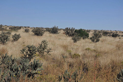
FIGURE 26-27 Two species of plants are abundant and readily available here, but mammalian grazers such as deer, prong-horns, and buffalo will not eat the cactus under any circumstances. It would be nutritious, but its spines are too strong of a defense. The grazers will eat only one prey (the grass) while completely ignoring the other (the cacti).
At this point botanists and zoologists diverge greatly. Animals are heterotrophs and their diets must include both energy and nutrients, and of these, energy is of special significance. It is typically the central factor in theoretical studies of optimal foraging theory performed by zoologists. Plants are autotrophs, and although they also need both energy and mineral nutrients, their growth is most often limited by scarcity of minerals or water. Almost all plants have plenty of sunlight and thus plenty of energy, so it often catches botanists by surprise that zoologists focus so heavily on energy. Animals have much greater need for energy: They must generate heat and also move, not just flying, running, swimming, or crawling but also their organs move as they chew, swallow, and breathe.
Optimal foraging theory has produced an optimal diet model that makes four predictions. First, predators should prefer whichever prey yields the most energy per unit of handling time. Second, if the high-yield prey become sufficiently scarce, then the predator would be more successful by broadening its diet to include prey that are lower in energy if they are abundant and easy to handle. Third, some prey items will always be eaten if they are encountered, others will never be eaten even if easy to obtain, for example if the edible parts are not worth the trouble of overcoming the plant’s defenses. Fourth, the probability that a particular plant will be eaten depends partially on the abundance of other plants that are easy to handle and have higher value: Less profitable prey will be ignored if more profitable prey is available (FIGURES 26-27 and 26-28). Point #2 is especially important for plants that are prey items for omnivores, animals that consume both animals and plants. Animals are generally more valuable prey items than plants because they are high in protein, fat, and minerals whereas plants tend to be high in fiber and water but low in nutrients, unless the omnivore is eating fruit, seeds, or tubers. But even these plant storage organs tend to be low in protein and essential fatty acids, mostly providing just starch. Consequently, if high-yielding animal prey are abundant, an omnivore may completely ignore plants, not bothering with them even when they are easily available. But animal prey respond adaptively to predation by hiding or fleeing to a safer area. As these high-priority prey become more difficult to capture, omnivorous predators will turn their attention to plants as prey. Many studies have given results consistent with the optimal diet model and optimal foraging theory.
Competition Between Species
Several species often compete for the same resources; this is interspecies competition as compared to intraspecies competition discussed in Chapter 25. One plant species competes against other plant species for light, water, and minerals among other things. Even though various species have different niches, most niches overlap at least somewhat with other niches. If two species are competing, one or both grows or reproduces more poorly than it would if it had the entire habitat to itself. In exploitation competition, resource competition occurs when the organisms actually consume a shared resource, thus making it less available for other organisms. In interference competition, one organism restricts another organism’s access to resources even though the first might not be using it. For example, bracken ferns (Pteridium aquilinum) produce large leaves up to 3 m long that emerge from a subterranean rhizome on petioles that are as much as 1 m tall. During summer, the leaves are healthy and undergo resource competition for light, using light such that shorter plants below these large leaves have less light available. During autumn and winter, the dead leaves produce a thick layer of debris that lies on top of lower evergreen shrubs. The dead leaves do not use the sunlight but they prevent the shrubs from obtaining it, so bracken fern performs interference competition during winter (FIGURE 26-29).
FIGURE 26-28 (A) Early sailors often released several pairs of goats onto many small islands so that when the sailors returned in the following years, they could hunt the goats for food. While goat populations were low, the animals would eat whichever plants they preferred and ignore the rest. But if the returning sailors did not harvest enough animals, the goat populations increased so greatly that goats ate everything that was not too poisonous or spiny. Many islands became almost completely denuded. (B) At present, people are working to restore the natural communities of islands by removing goats. Fortunately, many plant species survived the goats by means of buried seeds, rhizomes, and bulbs, and plants are thriving again.
Mathematical models have been developed to study interspecific competition precisely, but these are more complicated than are needed here. The conclusions are that two competing species can coexist (one will not completely exclude the other) if each species has a greater negative effect on its own per capita growth rate then it has on the per capita growth rate of its competitor. Keep in mind that a population of individuals of a species never grows exponentially (Figure 25-23A) because as their population density increases, individuals interfere with each other and the population growth slows (the per capita growth decreases) at high density (Figure 25-23B). Two competing species can coexist in a community if each interferes with itself more than it interferes with the other. The second conclusion is that two species can coexist if one or the other can increase from low density even in the presence of the other. In other words, competition may drive a species to very low population numbers but if it is not eliminated completely, it will be able to persist in that sparse state or even increase. If a species can increase from very low population density even with its competitor present, then that species can be invasive (FIGURE 26-30). If its seeds or spores can somehow be distributed to a new community where its competitor is already established, those few seeds or spores will establish an initial low population that can survive and increase despite interspecific competition.
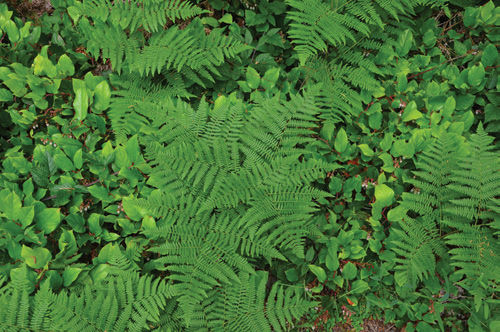
FIGURE 26-29 These are relatively small leaves of bracken fern, Pteridium aquilinum, but their long petioles raise the blades above the low shrubs (the stems of bracken ferns are subterranean rhizomes, only the leaves emerge above ground). The leaves catch and use sunlight, so this is exploitation competition; the leaves die and collapse in winter and create a dead layer on top of the evergreen shrubs. During winter, the leaves block sunlight but do not use it, so that is interference competition.
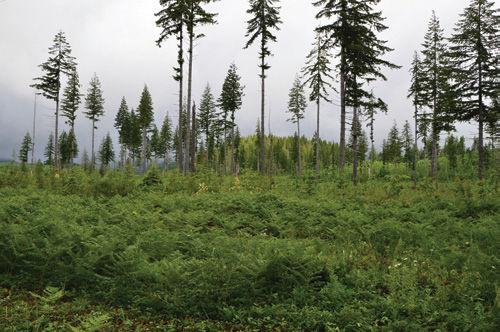
FIGURE 26-30 Bracken fern is such an intense competitor that it frequently takes over entire areas as its leaves catch sunlight above the short-stature shrubs and the stem spreads underground below them. Even when a tree seedling finally succeeds in growing through the leaves and reaching sunlight, its shade does not harm the bracken significantly because it photosynthesizes well in both dim light as well as strong light.
As several species compete for a resource, they use that resource and it becomes more scarce. Even a population of just one species growing without competition consumes resources and depletes them. One definition is that a resource is any substance or factor that can lead to increased growth rates as its availability is increased and that is consumed by an organism. Examples of abiotic resources are light, water, minerals, and space, and of biotic resources are the attention of pollinators, seed dispersers, and mycorrhizal fungi. Factors such as temperature are not resources because they are not consumed, and typically no plant uses so much carbon dioxide as to lower its atmospheric concentration enough to affect other plants, so even though it is consumed, it is not an item of competition. FIGURE 26-31 shows that as time progresses (bottom axis from left to right), a population grows; as it does so it consumes the resource, which consequently decreases with time. Why does the population density stop climbing, and why doesn’t the resource drop to zero? On the right side of the graph, the resource has dropped so low that it is now limiting the growth of the population. Ideally this occurs where the population density is such that its per capita birth rate matches is per capita death rate, so the population is neither increasing nor decreasing. This level of the resource is designated as R*; it is the minimum equilibrium resource needed to maintain a consumer population.
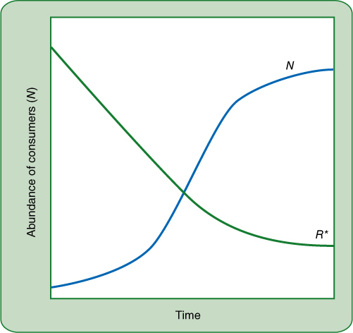
FIGURE 26-31 As a population lives in a habitat, it consumes and depletes resources. The model here postulates that the population will not increase so greatly that it completely eliminates the resource, although that is theoretically possible. Here, as the resource drops low enough, population growth slows and remains at a steady state. For this to occur, new resource must be added, as for example more nitrogen is added by nitrogen-fixing bacteria or by decomposition dead organisms.
If we consider two species, N1 and N2, that compete for this resource, we might expect that the species with the lowest R* (let’s say N1) would outcompete N2 and would eventually eliminate N2 from the community. As the two use the resource, its abundance decreases until it is below the R2* of N2, so there is no longer enough for N2 to produce offspring as fast as plants are dying. But the resource level is still above R1*, so the population of species N1 can still increase, driving the level of the resource even further below R2*. This is the underlying cause of the composition of many communities: They are lacking species that cannot compete against those already present and using the resources.
But there are many cases in which one species grows better than the other when the resource is low, but it does poorly when the resource is high, as in FIGURE 26-32. Notice that the growth curves for N1 and N2 cross each other. On the left, when the resource is high, N1 grows more rapidly than N2, but as the resource continues to drop near the middle of the graph, N1 grows more slowly than N2. This graph is based on time, such as the progression from spring to summer, and might represent a resource such as sunlight. In early spring, trees are leafless and sunlight is strong at the forest floor; species such as wildflowers that tolerate bright light flourish. But as trees leaf out a few weeks later, the forest floor has less light available, so wildflowers will suffer whereas any plants that are adapted to low light, such as mosses and ferns, will now thrive. In the following springtime, the situation will reverse itself.
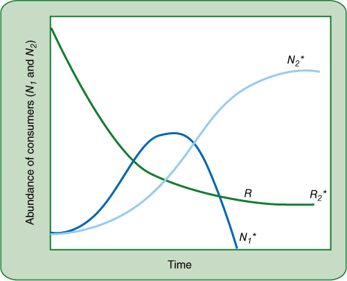
FIGURE 26-32 The growth of two consumer species, N1 and N2, competing for the same resource. The resource drops as would be expected, but at some point it will become too scarce to support the growth of one species (N1 here) that needs the resource in relatively large amounts, but the other species will continue growing if it is adapted to survive on low amounts of the resource.
Apparent Competition
Plants often face the problem that many herbivores will eat a variety of plants. In this case we say that the prey species share a predator. If all prey populations are low, then the population of the predator is probably low also. If something should cause the population of one of the prey species to increase, for example if the weather changes or mineral pollution acts as a fertilizer in a stream, that may cause the predator population to increase also. Even if the predator prefers one species and consumes other plants only incidentally, the larger predator population results in more herbivory on many plant species. Thus an increase in one plant species is associated with a decrease in others, and they appear to be in competition. Because the plants are not actually competing for and using a resource, this is called apparent competition.
![]() Beneficial Interactions Between Species
Beneficial Interactions Between Species
The various organisms within a community often interact in ways that are beneficial. If two organisms interact such that both benefit, that is mutualism or a mutualistic relationship. Familiar examples are pollinators and the plants they pollinate. If a plant’s flowers absolutely require an animal to carry out pollination, then that plant benefits greatly from the presence of its pollinator whereas the pollinator also benefits through the nectar or pollen it consumes during pollination. These two organisms are not preying on each other nor are they competing. If one organism helps another without receiving any benefit, that is a facilitation, the first organism facilitates the presence of the other. The beavers mentioned earlier are facilitators by building dams and creating ponds; the ponds are of great benefit to many plants and animals, but none of those really help the beavers.
The concepts of mutualism and facilitation are easy to understand intuitively, but whereas we have developed good mathematical models of negative interactions such as predation and competition, quantitative models of beneficial interactions are less well-developed. As a first step, we might expect that the Lotka-Volterra model could be changed from negative interactions to beneficial ones simply by changing certain negative signs in the equations to positive signs. The result is often that such equations then predict that both species in a mutualistic relationship continue helping each other such that both populations grow to infinity. Obviously, that never happens. Other factors that are not present in the equations prevent unending, infinite growth. The opposite situation, in which competition or predation drives one or both species populations to zero occurs everywhere; that is the fundamental reason why a community may be rich in species diversity but it is never infinitely rich. Competition and predation in every community prevent thousands of species from surviving in the community, otherwise virtually all species would live everywhere.
Even without mathematical models, basic concepts of beneficial relationships can be analyzed. Certain mutualistic interactions may have evolved from interactions that were initially predation. Pollination is a good example. The ancestors of angiosperms were wind-pollinated, as are conifers and many other plants even today. Insects would have preyed on the ancestral flowers by collecting and eating pollen. In many cases this would simply be predation with no benefit to the plant at all. But at some point, some insects began to visit the ancestral flowers regularly enough that insect pollination was as effective as wind pollination, and the plants began to benefit. At this point, evolution could favor the development of a mutualistic relationship in which certain plants became adapted to particular pollinators and vice versa. Other mutualistic relationships also may have begun as predator—prey relationships, for example nitrogen-fixing bacteria may have simply been pathogenic bacteria before root nodules evolved; mycorrhizal fungi also may have been pathogens before the mutualistic exchange of phosphate and carbohydrates evolved.
Although mutualisms are beneficial for both organisms, both organisms each incur a cost: The relationships are not free. Flowers have the cost of either producing nectar or losing pollen that is eaten; similarly, plants must supply carbohydrates to the nitrogen-fixing bacteria or to the mycorrhizal fungi. And the same is true in the opposite direction: Pollinators must work flowers to obtain nectar or pollen; bacteria and fungi must give up part of their fixed nitrogen or phosphate. Natural selection favors organisms that reduce their costs, and in the case of mutualists, this means that cheating can evolve. Cheating here refers to obtaining benefits without paying costs. Certain nectar-robbing bees bite through petals and easily obtain nectar without having to struggle around the stamens and becoming dusted with pollen. The nectar robbers fly from flower to flower without carrying any pollen, and the flowers lose their nectar without receiving the benefit of pollination. The ultimate fate of this short-circuited mutualism will depend on other species. If no other bees carry out pollination, then the flowers will be unable to reproduce and the plant species will die out in the area. The nectar-robbing bees will then be without a food supply unless they can switch to another nectar source. If another species of bee carries out enough pollination to ensure the plants’ survival, then the nectar-robbing is just another cost of living for the plant, but we might expect to see the evolution of thicker petals that are so tough the nectar-robbers cannot bite through them.
The concept of minimizing cost is also demonstrated in several cases of mycorrhizal associations and of symbioses between root nodules and nitrogen-fixing bacteria. No cases of cheating are known, but many of the plant partners in these mutualisms are able to break off the relationship if the soil is so rich that it is less expensive for the roots to obtain phosphate or nitrogenous compounds on their own. An especially sophisticated example was studied in yellow bush lupine (Lupinus arboreus) and Rhizobium bacteria. Some strains of Rhizobium fix nitrogen rapidly and transfer relatively large amounts to the legume root; others fix and transfer less. Scientists grew multiple plants of L. arboreus and infected some roots of each plant with a high-producing strain of Rhizobium; other roots of each were infected with a low-producing strain. Each L. arboreus plant produced larger nodules on roots infected with high-yielding Rhizobia and produced only smaller nodules on roots infected with low-yielding Rhizobia. Each plant allocated more resources (built larger nodules) where that investment was gaining the greatest reward. Mutualistic relationships are often described in rather human terms of each organism helping the other, but natural selection favors mutations that reduce costs and maximize benefits. Mutualistic relationships will be selected for only as long as the benefits outweigh the costs.
The concept of facilitation is a bit more difficult to conceptualize. It has been defined as an interaction in which one species alters the environment in a way that enhances the survival and reproduction of a second, neighboring species. Nurse plants are an example; these are plants that alter a small area of habitat immediately below themselves such that it is more favorable to the survival of seedlings of other plants as compared to other nearby areas not below the nurse plant. An example that is frequently cited is spiny desert shrubs (FIGURES 26-33 and 26-34). Seeds that germinate beneath the nurse plant are more likely to survive because the nurse plant provides shade as well as protection from herbivores that are deterred by the nurse plant’s spines. Seeds that germinate just a meter or two away from a nurse plant may be located in full, harsh desert sunlight and have no protection from herbivores. After a seedling under a nurse plant becomes established, it may grow so large that it emerges above the nurse plant, dwarfing it and perhaps even killing it. The problem with the concept of nurse plant is that it applies so broadly to so many organisms. A patch of moss provides a moist, airy seedbed for many seedlings; the shade of a forest facilitates the presence of shade loving ferns (FIGURE 26-35).
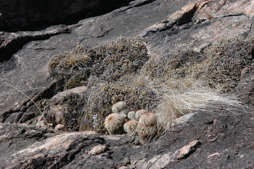
FIGURE 26-33 What appears to be a coarse moss here is actually Selaginella pilifera, a small lycophyte that grows even on bare granite boulders. Along with it are a small cactus, Echinocereus pectinatus, and several clumps of grass. The Selaginella forms mats that catch and hold rainwater as well as bits of windblown soil, both of which would be helpful for the cactus and the grass. In this area of central Texas, E. pectinatus almost always grows in clumps of Selaginella—undoubtedly, the tiny, delicate cactus seedlings survive better in the mats of Selaginella than they do on bare rock. But at some point, they outgrow the need for the Selaginella and can survive even if the Selaginella were to die. The cactus needs the nurse plant only while it is very young.
Facilitation plays a role in succession, especially primary succession in which organisms become established on newly created substrates. For example, volcanoes produce new substrate in the form of lava flows or ash fields that are completely sterile as they cool (FIGURE 26-36). Similarly, as a glacier advances, its ice scrapes away all soil and organisms such that when the glacier later retreats, the exposed soil is free of all organisms. In both cases, there is usually little or no soil at all. Certain pioneer species such as mosses and lichens are able to colonize bare rock; others must be able to insert slender roots into the tiniest of cracks. All pioneers must tolerate very low levels of nutrients, especially low amounts of nitrogenous compounds. Many pioneers have mutualistic associations with nitrogen-fixing bacteria. As the pioneers grow, they shed leaves, bark, and fruits, contributing organic matter to the habitat. Much of the litter will become the substrate for fungi, which now are able to survive in the habitat and become new species in the community. The rest of the debris will collect in cracks and crevices along with dust, thus creating small pockets of soil in which non-pioneer species can survive. Each set of organisms in this primary succession alters the habitat and facilitates the survival of the next set.
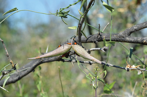
FIGURE 26-34 The two large horn-shaped pods are the fruits of a milkweed vine (Asclepias) that grows by twining upward on the trunk and branches of a mesquite tree (Prosopis). The mesquite produces an abundance of spines; by growing on mesquite, the milkweed vine receives both protection and support.
We still have little experimental or theoretical knowledge about the ways in which beneficial interactions affect community diversity. This is an area in which a great deal of research remains to be done.
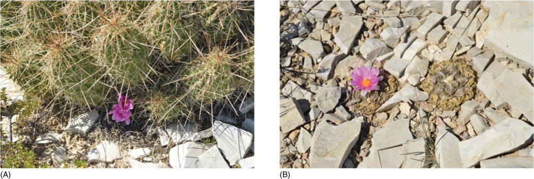
FIGURE 26-35 (A) The large spiny cactus is a hedgehog cactus (Echinocereus engelmannii) but the flower belongs to a small, spineless living star cactus (Ariocarpus fissuratus). The spines of the hedgehog cactus provide a safe, protected site for the smaller cactus, and it would appear that this is a case of the large spiny plant being a nurse plant for the spineless Ariocarpus. (B) Ariocarpus is much more plentiful in open sun, away from the shade of the Echinocereus. The proximity of the two is just incidental, this is not an example of a nurse plant.
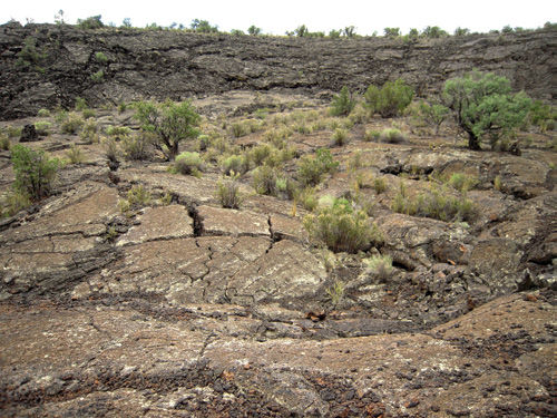
FIGURE 26-36 The substrate of El Malpais National Monument just west of Albuquerque, NM, is lava less than 3,000 years old. The only soil present has mostly blown in from other areas, only a tiny amount has weathered off the rocks in such a short period of time. Lichens can live on the bare rock surface, but few true plants of any sort can. There are a few small ferns growing in deep cracks where there is protection from sun and where rainwater collects. Likewise, the seed plants present—pinyon pine and Apache plume—grow only if their roots reach small pockets of wind-blown soil.
![]() Metapopulations in Patchy Environments
Metapopulations in Patchy Environments
If all individuals of a species were able to interact freely, we would speak of just one population rather than of several. The world is patchy and heterogeneous; it contains many areas suitable for any particular species, but those areas are physically and geographically separated from each other. For example, hardwood forests suitable for maples are widespread but separated into numerous discrete forests; the maples in one constitute a population distinct from the populations of maples in other forests. If several local populations are interconnected by migration and gene flow between the patches, the local populations constitute a metapopulation. In conservation biology, with the goal of preserving endangered species, the concept of metapopulations is crucial. We must consider all the populations of a species, not just one or two in which a species appears to be doing well.
A common model of metapopulations makes four assumptions:
1. A region of the environment is composed of many discrete patches in which the species can live.
2. Some patches are occupied by the species whereas other suitable patches are not.
3. Empty patches will become colonized by migration from occupied patches.
4. Populations within individual patches have a probability of going extinct within that patch.
Let’s examine these more closely. The various patches will be separated from each other by varying distances, and some patches will be larger than others. In some patches, most critical parameters for the species are optimal or nearly so, and the species thrives there; these are high-quality patches. But other patches have one or several suboptimal parameters; the species does poorly in such low-quality patches. Some low-quality patches maintain their population of the species only because new members migrate in from high-quality patches rapidly enough to offset the loss of existing members (FIGURE 26-37). The high-quality patch is a source habitat, and the low-quality one is a sink habitat. For animals, migration from one patch to another can be by flying, walking, or swimming and so on; for plants it is by the dispersal of seeds or spores.
Point #2 postulates that some patches are occupied by the species, others are not. Population sizes always vary with time due to predators, competition, and disturbance. At certain times, many individuals are present; at other times there are only a few, and sometimes the species may die out in a particular patch. But the species as a whole might still be very healthy as long as other patches have adequate populations and at least a few individuals are colonizing empty patches and establishing new populations.
This point is particularly important for conservation biology: Empty patches are not surplus or spare or unneeded. The biology of some species involves numerous local populations that are ephemeral: Any particular population thrives for a certain amount of time but then dies off. Perhaps it is outcompeted or perhaps it is a species that does well early in succession but poorly later in succession. The success of the species depends on its being able to colonize empty patches at least as quickly as it dies out in occupied patches. As long as there are unoccupied patches where new populations can be established, the species is healthy.
Imagine a conservation program planning to establish wildlife preserves to maintain an endangered species. The planners should set aside not only patches that are currently occupied by the species but also several that are unoccupied so that the species can later colonize them as part of its natural cycle. If the species is one that thrives early in succession but poorly later on, then any preserve that now contains the species will automatically change through succession such that the species is excluded. Preserve managers would need to work to counteract succession; they would need to constantly eliminate competitors and restock needed individuals. Similarly, planners might inadvertently set aside a low-quality sink habitat without preserving the needed high-quality source habitat; if so the preserve will fail.
FIGURE 26-37 El Capitan Peak in Guadalupe Mountains National Park, located on the border between Texas and New Mexico, is the only high altitude area within hundreds of miles. This small area of alpine habitat, surrounded by desert vegetation, is not large enough to sustain many of the species of its high altitude plants, but populations of them persist because larger alpine habitats only a few hundred miles away contribute seeds and spores.
Point #3 emphasizes the need for colonization of new patches by migration. It is easy to think of migration as birds flying from one patch to another and establishing new nests anywhere they please. But birds are often extremely careful about where they fly: Some fly only within the dense cover of forests, others fly over grassy areas where they can see mice or other prey. Other animals too are particular about the terrain and vegetation they will visit. Plants migrate by means of their seeds or spores. These may be blown by wind or carried by animals, caught in fur or feathers, or carried inside their digestive system. Consequently, the propagules of some plants move very long distances in short times and can colonize widely separated patches. Other plants have seeds that fall close to the parent plant or are dispersed by ants; such plants migrate slowly.
Migration corridors that interconnect patches are important. Corridors may be narrow but must have proper food, water, and places for hiding or nesting. Natural migration corridors seem to better than artificial ones, so in planning wildlife preserves and mitigating habitat fragmentation, it is better to preserve natural areas for corridors rather than attempt to construct artificial ones (FIGURE 26-38). One of the most extensive natural migration corridors is the series of national parks and national forests that interconnect virtually all the alpine regions of the Rocky Mountains from New Mexico to Canada. On a smaller scale, we now leave strips of forest or grassland, whichever is appropriate, to interconnect larger forest preserves. Highways are severe barriers that kill many animals that risk crossing them; in some areas we now construct wildlife bridges across highways to provide safe passage for animals (see Figure 26-7A). In other areas, the protected animals may prefer tunnels under the roads: Some animals prefer to have protection overhead; others prefer open sky. Migration corridors have several negative consequences: They allow the migration of predators, competitors, diseases, and exotic species as well as the migration of protected ones.
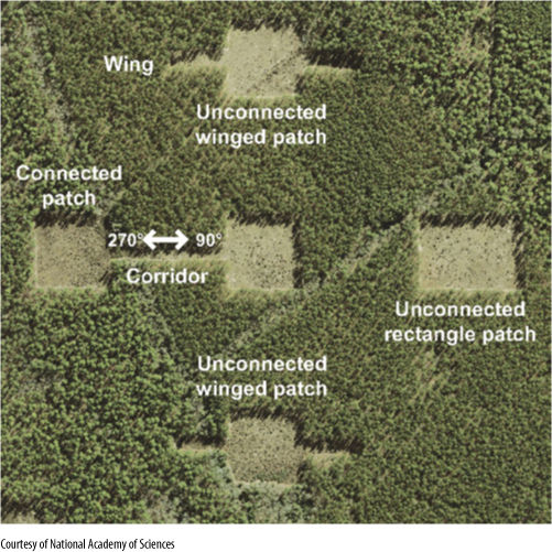
FIGURE 26-38 This is a study site designed to determine the effects of various types of migration corridors. It contains both connected and unconnected patches; some patches have wings that resemble corridors but do not lead to another meadow habitat.
Point #4 postulates that populations within a patch have a probability of going extinct locally. For some species this probability is low and the species persists for many generations in most patches, but for other species the probability is high and the species occupies a patch only briefly. A fugitive species is one that survives by colonizing new patches, flourishing temporarily, and then colonizing more patches before it dies out in old ones. Many weeds of disturbed sites are fugitive species (FIGURE 26-39).
Migration between patches is becoming increasingly important due to global warming. As Earth’s temperature rises, habitats in general are becoming warmer. Those near the equator may become too warm for many species that are adapted to them now, whereas habitats closer to the poles may become warm enough to be suitable. A recent study of the ranges of many species found that on average, the ranges have been shifting toward the poles by 6 to 17 km per decade for the last 50 years. If species are to survive, they will need to migrate poleward, moving from patch to patch. But for many species, each new warm, unoccupied patch is separated from the nearest occupied patch by inhospitable terrain, such as farms, roads, cities, or industrial areas. For many species, either no natural migration corridors exist or they have been disrupted by human activity. One proposed solution is assisted dispersal (also called assisted migration), in which animals are captured in one area and released into the new area. For plants, either seeds or whole plants can be moved. Assisted dispersal carries a large risk: It will be difficult to know which regions truly are newly-formed appropriate patches, patches that the species would have colonized if it could have. Even if the patches we select for assisted dispersal are appropriate, we are still artificially introducing a foreign species.
FIGURE 26-39 Tumbleweeds (Salsola kali) are typically the very first plants to germinate in disturbed sites such as beside newly built roads and construction sites, at least in the western United States. They often completely fill a disturbed area in the first year or two; after that, other species germinate and crowd them out. By that time, they will have spread their seeds to other newly disturbed sites. Although they are never present in any patch for long, they are extremely successful throughout the western states.
![]() Interconnectedness of Species: Food Chains and Food Webs
Interconnectedness of Species: Food Chains and Food Webs
The simplest communities typically have at least three trophic levels: primary producers (plants, algae, cyanobacteria), primary consumers (herbivores), and secondary consumers (carnivores). For example, a prairie might consist of several species of grasses and herbs that are fed upon by mice and deer, which in turn are prey to bobcats or coyotes. If environmental conditions are very harsh, as in deserts or high alpine areas, the populations of primary produces are sparse and consequently the populations of herbivores will be sparse as well. With so few herbivores, only a single species or two of carnivores can be supported, and the community has only three trophic levels. In areas with better conditions and more luxuriant plant growth, enough energy may be available to support numerous species of herbivores and omnivores, and in turn there may be high species diversity of carnivores, some of which prey only on other carnivores. Such a community has more than three trophic levels.
We can study species interactions across trophic levels in several ways. The simplest is to choose one predator, then identify its main prey and the plant species that supports them. This direct line of consumption would be a food chain. But most carnivores eat a variety of prey, and those prey may be herbivores, or omnivores, or other carnivores. Similarly, most prey species will be threatened by multiple carnivores. If we trace all the prey of the top carnivores, and then trace the food sources of each of those prey species and so on, we obtain a network of numerous interrelationships called a food web. At the first stage of our study we might merely attempt to make a map of who feeds on whom. But each of the organisms have favorite food sources, so we might attempt to map out which herbivores consume the most energy, and in turn which are eaten the most, etc., so as to trace how energy flows through the community. This would be an energy flow web; it is extremely difficult to construct energy flow webs for real communities.
It is common to see diagrams of food webs and energy flow webs in textbooks of biology and ecology. But in fact those are primarily just for illustrating relationships and most have severe problems. The majority of studies of food webs are very incomplete, giving their primary attention to large familiar animals such as carnivorous mammals, birds, fish, and reptiles; less attention is given to herbivorous mammals such as deer and mice, and little attention is paid to plants. However, a few studies have shown that invertebrates such as ticks, lice, flies, mosquitoes, and caterpillars make up as much as 50% of the biomass of a community. But typically these are never studied; they are not even identified to genus or species. Similarly, studies of aquatic food webs often identify the primary producers merely as “algae” with no effort given to distinguishing one species from another.
It is difficult to trust food web studies knowing that they are so incomplete, but a few cautious conclusions can be drawn. Most communities have a small number of strong food chains through which most energy flows and a much larger number of other food chains involving much less energy. However, the abundance of low energy interactions among many organisms tends to stabilize communities. In general, communities with high diversity seem to be more stable than those with low diversity.
The incompleteness of many food web studies appears to be less of a problem than we would expect at first. Certain species can be removed and seem to have little effect on most other members of the community; consequently, detailed studies of most members of a food web would not provide much useful information. In contrast, the presence or absence of certain species, called keystone species, dramatically affects the structure to their community. A keystone species has an impact out of proportion to its size or the number of individuals present. For comparison, a dominant species, such as a particular grass of a prairie or a tree of a forest, will have a strong impact on the structure of a community, but that impact is related to its abundance. It is easy to recognize the dominant species of a community, but it is very difficult to identify a keystone species without actually removing the species to examine how much it affects community structure.
A classic example of a community with a keystone species is seen in the relationships between sea otters, sea urchins, and kelp “forests” (FIGURES 26-40 and 26-41). Sea otters were hunted almost to extinction in the northern Pacific Ocean, and were finally given protection from hunting in 1911. Sea urchins are a favorite food of sea otters, and during the time while sea otters were hunted to low populations, sea urchins thrived due to low predation. They would scour rocky coasts, eating various algae, especially sporelings of kelp (Macrocystis). During a trip to the shore, one would encounter numerous urchins in a barren, desolate wasteland. But after 1911, sea otter numbers increased and they reduced the populations of sea urchins. With urchin grazing minimized, kelp spores could germinate and grow into giant plants, creating extensive, dense underwater forests. A kelp forest, much like a terrestrial forest, is a complex habitat; fish can feed and hide among the kelps, epiphytic algae can attach to kelp, and so on. Sea otters are a keystone species: By protecting them and letting their numbers rise, sea urchins were reduced, and the coastal communities became much more productive, much richer, and the number of species present increased dramatically.
FIGURE 26-40 Sea otters prey on sea urchins, keeping their numbers low, and thus reducing the amount of grazing the sea urchins do.
FIGURE 26-41 If sea urchins are abundant, they eat young plants of kelp before they can become established. But if sea urchin populations are kept low, then kelp spores grow into large plants, creating “kelp forests” that are complex and nourish many species of organisms.
Recognizing a keystone species is relatively easy if it is removed and then restored, as were sea otters. But it is extremely difficult to recognize a keystone species on the basis of studies of either food webs or energy flow webs. We are in a dilemma now because throughout human history, we have worked to exterminate predators that could harm us and our livestock: We have greatly reduced the numbers of large cats (lions, cougars), carnivorous birds (eagles, hawks), bears, wolves, and so on. Almost certainly some were keystone species that kept herbivore populations low and allowed plant diversity to be high. Unfortunately, they were removed before we had made any substantial studies of community structures, so we have no way of knowing how altered our present communities are without them. Unfortunately, we have also replaced most natural herbivores with cattle, sheep, and goats, so most communities are now far from natural. We are at present trying to rebuild natural communities in some areas. Herds of bison were preserved in Yellowstone National Park, Caprock Canyon State Park in Texas, and several other areas. Grizzly bears have recently received protection in certain areas, and most recently wolves have been reintroduced to the northern national parks in the Rocky Mountains. As anticipated, the wolves immediately lowered the population of elk, which had become so abundant they were overgrazing and degrading much of the parks. An additional benefit is that the presence of wolves is causing the elk to change their behavior, spending more time in the protection of forests and less time in open meadows and along streams where they would be vulnerable to attacks by wolves. With reduced trampling by elk, meadows and stream banks are now recovering and developing a richer diversity of plants, and populations of willow and aspen are increasing. Stream erosion is greatly reduced, and these trees are used for nesting by birds and as construction material and food by beavers. The number of beaver ponds has increased, creating more habitat for fish, otters, amphibians, and marsh plants. Coyotes consume large amounts of small animals such as mice and rabbits, but the wolves have reduced the populations of coyotes, leading to an increase in rabbits, mice, and others, which benefits hawks and eagles. The removal and then reintroduction of a single species is having a dramatic effect not only on the animals of Yellowstone, but also on the plants and on shapes of creeks and rivers.
Part of the complexity of community ecology is that many animals can and will change their behavior depending on which other species are present. The behavior of elk and wolves is one example and illustrates how difficult it would be to predict the response of an entire community based only on artificial experiments involving isolated factors. Another example of a change of behavior and its unpredictable consequences is provided by grasshoppers, spiders, and plants. Grasshoppers are a major herbivore in old fields, and one (Melanoplus femerrubrum), prefers to eat the grass Poa pratensis (Kentucky bluegrass). Due to grasshopper herbivory, a competing plant, Solidago rugosa (goldenrod), is able to thrive. A spider (Pisaurina mira) is a predator of the grasshopper; when present, it reduces their numbers somewhat. But just as importantly, when grasshoppers detect the presence of the spider, they alter their behavior by switching from feeding on the grass to the goldenrod. Spiders are more likely to hunt in grasses than in the goldenrod, so grasshoppers are safer by switching their plant food. As a result, if spiders are present, goldenrod suffers more grasshopper predation and its population decreases, whereas if spiders are absent, grasshoppers switch from goldenrod to their preferred food Poa pratensis, lowering its numbers. Thus the balance between Poa and Solidago is determined to a large degree by the presence or absence of the spider, which eats neither one of them.
Community ecology is a very young science, and just a few basic principles have been established. Much is left to be learned; there is much we do not know. But we are still burning fossil fuels, adding greenhouse gases to the atmosphere, and causing Earth’s climate to change. We have initiated a worldwide experiment in altering communities everywhere. We need to improve our understanding of community ecology as quickly as possible in hopes of preventing major environmental disasters.
Plants and People
BOX 26-2 Some Laws to Protect Species Have Harmful Consequences
Treaties to protect endangered species often do more harm than good. In 1975, the Convention on International Trade in Endangered Species (CITES) was proposed and ratified by many nations. This treaty has a noble purpose: to control, and in many cases to completely eliminate, international sales of endangered species. Until 1975, there was an almost completely open market on animals and plants, whether they were as abundant as bananas or as rare as a black rhinoceros. Live animals could be captured and then sold to zoos anywhere in the world, or much worse and much more profitable, they could be sold to private “game ranches.” Hunters on these ranches could pay to hunt and kill elephants, giraffes, monkeys—anything. An even larger problem is that various animal organs are highly valued: elephant ivory, rhinoceros horn, hides, and internal organs. Some were valued for their beauty, others for reputed medicinal properties, and still others were believed to be either aphrodisiacs or enhancers of male virility. Unknown numbers of animals were killed, butchered for parts in the field, and the corpses left to rot.
The goal of CITES was to regulate this trade. Some animals were judged to be sufficiently plentiful that some “harvesting” could be allowed; others were so endangered that they were to be left unharmed and the harvesting quota was set at zero. Individual countries tried to control this, but if some countries still allowed these to be purchased, smugglers would find a means of obtaining the animals from their habitat. With CITES, all countries agreed to control trafficking in endangered species, so if illegal products are discovered in cargo anywhere, they can be seized. This makes smuggling much more difficult, but of course it still exists; it is common for game wardens in Africa to find corpses of elephants without tusks and rhinoceroses with their horns cut off.
Unfortunately, the people who wrote CITES decided to protect plants but without taking into consideration that plants are different from animals. CITES controls the international trade in whole individuals and also their part (hides, horns, tusks, testicles) because harvesting parts usually kills the animals. But plants are different: Harvesting a portion of a plant’s seeds does not harm the plant or the seed crop, and for many plants, it is safe to take cuttings that can later be rooted and grown as a new clone of the original plant. In fact, by collecting a portion of the propagules, the endangered species can be propagated in botanical gardens or planted in new safe areas, making the species a bit less endangered. Unfortunately, CITES does not recognize this: Both whole individuals and their parts are banned, for both animals and plants.
CITES has greatly hindered the legitimate work and research of zoologists and botanists. Prior to CITES, a biologist would usually work in cooperation with local biologists to explore remote, poorly known parts of the world. Part of the research would be to collect specimens for propagation in university research gardens. If sufficiently plentiful, some living material would be given to professional propagators—nurseryman—who often could turn a few seeds or bulbs into tens of thousands of plants that could be sold worldwide. Many people could enjoy the new, exotic species without any harm to the original plants.
CITES has a provision for scientific collectors but it is difficult to use. A person going from the United States to another country to study biology, for example to Latin America, Africa, or Southeast Asia, must apply for permits both from the U.S. and from the host country. The application must list the exact number of individuals of each species to be collected—a difficult task when exploring for new undiscovered, unnamed species. Until recently many of the less-developed countries did not have an agency, not even a single agent, who could approve such an application and provide the needed permit.
Another problem with CITES and plants is that border inspection agents can quickly learn to recognize an elephant tusk, a rhinoceros horn, a leopard hide, but they cannot quickly learn which of the hundreds of orchids are endangered and which are plentiful, so all orchid species are treated as endangered and require permits. The same is true of cacti and bromeliads.
Additional trouble has been caused by the convention on biological diversity that was adopted in Rio de Janeiro in 1992. The background of this treaty is that we had come to appreciate the value of medicinal plants: If aspirin, vinblastine, and Taxol could be extracted from plants, what other life-saving drugs might exist in the untested, unknown plants of the world? Also, animal venoms often kill by interfering with nerve metabolism, but in the proper doses they give us an amazing control over various nerve functions. Teams of biologists were sent out across all parts of the world to obtain plant and animal samples to be tested for effectiveness against many diseases. Obviously, the best place to start is to talk to the local healer (curandero, witch doctor) of a village. Unfortunately, this exploration came at a time when many countries felt they were being treated as second-class citizens in the world: Americans and Europeans would arrive, collect samples, mine for minerals, drill for oil, pay a small amount and then later sell expensive medicine, expensive chemicals, and expensive gasoline and diesel. These countries were the driving force behind the Rio Convention, and insisted that it state that the organisms in a country are the patrimony of the country. That is, the organisms, their DNA, their descendants, and any medicines derived from the organisms belong to the country of origin. A typical collecting permit would stipulate that (1) the researcher could not ask anyone if a plant or animal has medicinal properties, (2) could not extract DNA from any organism, (3) could not propagate the organism, and (4) must completely destroy the entire organism, DNA, and tissue samples when the research was completed. This severely suppressed research and hindered efforts to save endangered plants and animals by means of propagating them in botanical gardens and zoos.
Since the passage of CITES, habitat destruction has accelerated. Millions of square kilometers of forests and grasslands have been and are being cleared for farms and ranches, to harvest lumber and paper, and to obtain valuable woods such as teak and mahogany. Cities and suburbs continue to sprawl wider and wider. Clearing a tract of land for farming or for housing kills all the organisms that had been present, whereas biological exploration and collecting would have saved some individuals. Both CITES and the Rio Convention need to be thoughtfully modified to stop the devastation and improve scientific discovery.
 At the Next Level
1. Succession and pioneer species. Until 12,000 years ago, all of Canada and much of the northern United States was covered by the Laurentide Ice Sheet. This was more than a mile thick in many places, and actually caused Earth’s crust under Canada to sink downward. Since the beginning of the Holocene warming 12,000 years ago, the ice sheet retreated, but this has been patchy because ice retreated at different times in different places: 11,000 years ago in the lowlands, more recently as glaciers continue to retreat in the mountains. Consequently the ages of communities in Canada and the mountains of the western U.S. vary between 12,000 years and zero years (at the foot of a retreating glacier today). It is possible to see older stages of succession as one walks down a valley formerly occupied by a retreating glacier. Succession in pioneer species has been studied extensively in these areas, and you should find many good summaries and original research papers.
2. Sky islands. The communities located on cool mountain peaks usually differ greatly from those in the warm lowlands between mountains. When Earth is very cool, the communities typical of mountain peaks may be able to survive in the lowlands, allowing communities of adjacent mountain peaks to interact and exchange species. Species normally confined to the cold high latitudes (far north in the northern hemisphere) may migrate far toward the equator. When Earth warms again, many species survive by occupying higher and higher altitudes on nearby mountains. As result, mountain tops near the equator may harbor species that are now separated from their relatives hundreds of miles away on other mountains, or thousands of miles away in cool lowlands at high latitudes. Thus, the tops of some mountains are considered “sky islands,” each having its own communities that evolve and adapt in isolation from related communities. In researching this topic be sure to include the concept of refugia (sing.: refugium).
3. Density compensation. An important concept in community ecology is the reaction that occurs if a particular component is changed. For example many communities have several plant species that produce small seeds (such as grasses) and several species of grain-eating (granivorous) rodents. If the density of one species of granivore is decreased (for example, by disease or by experiment), will the density of other granivores increase compensatorily (that is, such that the total biomass of granivores remains the same)? Or will changes in the density of one have no effect on the density of the others? This has not been resolved, and may not be the same in all communities, but this is a significant area for independent study.
4. Metapopulations and conservation biology. This chapter gave only a brief introduction to the concept of meta-populations, but this is very important when designing wildlife preserves for endangered species. You can study this further on your own with Internet searches. I recommend the book Community Ecology by Garry G. Mittelbach (2012, Sinauer Associates). It is an excellent text, well-written and well-illustrated.
SUMMARY
1. A community is a group of species that occur together at the same time and place.
2. Many communities undergo a more-or-less predictable sequence of changes called succession.
3. A community that remains more or less the same for many years is a climax community.
4. We humans are members of many communities, and we contribute to habitat loss, habitat fragmentation, and overharvesting, but we also contribute to community restoration and resource conservation.
5. When studying community diversity, the size of the area being studied, called its scale, is important; larger areas have more diversity than smaller areas.
6. In most communities, plants are the most important primary producers, and they are the prey for herbivorous and omnivorous predators.
7. The paradox of enrichment is a phenomenon in which fertilizing or enriching a community may lead to the loss of diversity rather than an increase in abundance of all species.
8. Fixed effort harvesting is a technique that automatically decreases harvests whenever a resource is in short supply or is endangered.
9. Multiple species can compete with each other for a resource; if they actually consume the resource and reduce it, it is exploitation competition. If one merely interferes with access to the resource by other species, it is interference competition.
10. Species of a community may interact such that one benefits (facilitation) or such that both benefit (mutualism).
11. Populations typically are separated by regions of unsuitable habitat; if species can migrate between the various populations, they all constitute a metapopulation.
12. Metapopulation ecology is important when planning the establishment of wildlife preserves; incorporating migration corridors may be essential.
13. Food webs and energy flow webs are the predator—prey relationships within a community, but studies of these webs are not able to incorporate or measure every possible relationship.
IMPORTANT TERMS
apparent competition
assisted dispersal
checklist
climax community
community
community restoration
energy flow web
exploitation competition
facilitation
fixed effort harvesting
fixed quota harvesting
food chain
food web
fugitive species
functional response
habitat fragmentation
habitat loss
interference competition
invasive species
keystone species
maximum sustained yield
metapopulation
mutualism
mutualistic relationship
nurse plant
optimal diet model
optimal foraging theory
paradox of enrichment
prey-dependent
primary succession
resource
sink habitat
source habitat
species abundance distribution
species-area relationship
succession
zero growth isocline
REVIEW QUESTIONS
1. Define a community. Do communities have sharply defined geographical boundaries? Explain.
2. Some communities change with time. What is that process called? Describe an example of it.
3. Other communities are more or less the same over long periods of time; what is the name for a community like that? Why does such a community remain the same?
4. We humans are members of many different communities. Describe some, and describe how we affect the biology of other organisms in some of these communities.
5. What is community restoration? Why is it necessary? Describe several examples.
6. How does habitat loss differ from habitat fragmentation? What is the importance of protected migration corridors?
7. What is a species checklist? Is it possible to use a checklist to determine which species are abundant and which are rare?
8. Scale is usually important in studies of community ecology; which has greater species diversity, larger plots or smaller ones? Why?
9. Tropical areas near the equator have higher species diversity than do temperate areas at high latitudes. Discuss several of the proposed causes. Be sure to mention the contribution of past global climate change.
10. Describe species abundance distribution. Draw several hypothetical ones, for example one in which almost all species are very rare, or one in which a few species are extremely rare but most are merely sparse and a few species are very abundant. Is it possible to draw a species abundance distribution graph in which almost all species are extremely abundant? (Hint: Is it possible to have a community in which two species are both so abundant that the members of each account for more than half the individuals within the community?)
11. In predator—prey interactions, do predators typically consume so much prey that the prey species is lost from the community? Or can the two species co-exist for a long period? Describe this.
12. If the rate of some process is governed by the abundance of prey individuals, we say that it is prey-dependent. Give some examples of prey-dependent processes.
13. The factors r and K were discussed in Chapter 25; describe each. The factors a, f, and q are presented here; describe each of these.
14. A prey population with a curved zero growth isocline is important because the zero growth isocline of the predator might intersect it to either the right or the left of the maximum value. One intersection will result in a stable interaction; the other will result in an unstable one. Which is which and why?
15. What is the paradox of enrichment? How are zero growth isoclines involved in this? Give an example of this in real life.
16. Fixed effort harvesting and fixed quota harvesting are two very different approaches to fishing, hunting, and timber harvest. Describe each and describe how each affects the population being harvested.
17. The optimal diet model makes four predictions; list all four.
18. What is the R* of a resource being used by a species? When two species, N1 and N2, compete for the same resource, how do their respective R1* and R2* affect the outcome?
19. Define mutualism. Give two examples of mutualistic relationships.
20. Once a mutualistic relationship evolves between two species, will natural selection and co-evolution cause the two species to become continuously more dependent on each other? Or is it possible for one to end the mutualism? Describe.
21. Describe primary succession. Do you think it may have been important in the last 12,000 years as ice sheets and glaciers retreated?
22. Animals migrate through the movement of whole animals (walking, flying). How do plants move? Describe several mechanisms.
23. The model of metapopulations postulates that some patches that are suitable for a species will not be occupied by the species. Does that mean that the patch is not really suitable after all? Does it mean that it is unimportant for the conservation of the species and can be used for industrial development? Explain.
24. The model of metapopulations also postulates that many species occupy their patches only temporarily, that sooner or later they will be eliminated by competition or some other factor. If this is true, would such a patch make a suitable wildlife preserve for that species? Discuss what wildlife managers might have to do with such a preserve.
25. In many cases, it is beneficial to have migration corridors connecting various patches of a metapopulation. Do you think it would be suitable to designate the shoulders of a busy highway as a migration corridor for deer (or any other timid animal) if that highway ran from one patch to another? Discuss.
26. What is assisted dispersal? Why might it be more important now than it has been in the past? Why do some people object to it?
27. Most studies of food webs do not bother with examining most of the species or even most of the organisms in the actual web. Why? How reliable are such studies? Are all organisms and all interrelationships equally important?
28. What is a keystone species? Describe an example.
Design Credits: Hummingbird: © Tongho58/Moment/Getty; Green plant cells: © ShutterStock, Inc./Nataliya Hora; Purple tulip: © ShutterStock, Inc./Marie C Fields; Dandelion: © ShutterStock, Inc./danielkreissl; Poppy: © ShutterStock, Inc./Saruri; Plant icon: © ShutterStock, Inc./Vector; Digging man icon: © ShutterStock, Inc./Z-art