CHEMISTRY THE CENTRAL SCIENCE

19 CHEMICAL THERMODYNAMICS

19.7 FREE ENERGY AND THE EQUILIBRIUM CONSTANT

In Section 19.5 we saw a special relationship between ΔG and equilibrium: For a system at equilibrium, ΔG = 0. We have also seen how to use tabulated thermodynamic data to calculate values of the standard free-energy change, ΔG°. In this final section, we learn two more ways in which we can use free energy to analyze chemical reactions: using ΔG° to calculate ΔG under nonstandard conditions and relating the values of ΔG° and K for a reaction.

Free Energy Under Nonstandard Conditions

The set of standard conditions for which ΔG° values pertain is given in Table 19.2. Most chemical reactions occur under nonstandard conditions. For any chemical process, the relationship between the free-energy change under standard conditions, ΔG°, and the free-energy change under any other conditions, ΔG, is given by

In this equation R is the ideal-gas constant, 8.314 J/mol-K; T is the absolute tempera ture; and Q is the reaction quotient for the reaction mixture of interest. (Section 15.6) Under standard conditions, the concentrations of all the reactants and product are equal to 1. Thus, under standard conditions Q = 1, ln Q = 0, and Equation 19.19 reduces to ΔG = ΔG° under standard conditions, as it should.

SAMPLE EXERCISE 19.10 Relating ΔG to a Phase Change at Equilibrium

(a) Write the chemical equation that defines the normal boiling point of liquid carbon tetrachloride, CCl₄(l).

(b) What is the value of ΔG° for the equilibrium in part (a)? (c) Use data from Appendix C and Equation 19.12 to estimate the normal boiling point of CCl₄.

SOLUTION

Analyze (a) We must write a chemical equation that describes the physical equilibrium between liquid and gaseous CCl₄ at the normal boiling point. (b) We must determine the value of ΔG° for CCl₄, in equilibrium with its vapor at the normal boiling point. (c) We must estimate the normal boiling point of CCl₄, based on available thermo-dynamic data.

Plan (a) The chemical equation is the change of state from liquid to gas. For (b), we need to analyze Equation 19.19 at equilibrium (ΔG = 0), and for (c) we can use Equation 19.12 to calculate T when ΔG = 0.

Solve

(a) The normal boiling point is the temperature at which a pure liquid is in equilibrium with its vapor at a pressure of 1 atm:

(b) At equilibrium, ΔG = 0. In any normal boiling-point equilibrium, both liquid and vapor are in their standard state of pure liquid and vapor at 1 atm (Table 19.2). Consequently, Q = 1, ln Q = 0, and ΔG = ΔG ° for this process. We conclude that ΔG° = 0 for the equilibrium representing the normal boiling point of any liquid. (We would also find that ΔG° = 0 for the equilibriarelevant to normal melting points and normal sublimation points.)

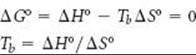
(c) Combining Equation 19.12 with the result from part (b), we see that the equality at the normal boiling point, T_b, of CCl₄(l) (or any other pure liquid) is

Solving the equation for T_b, we obtain

Strictly speaking, we need the values of ΔH° and ΔS° for the CCl₄(l)–CCl₄(g) equilibrium at the normal boiling point to do this calculation. However, we can estimate the boiling point by using the values of ΔH ° and ΔS° for CCl₄ at 298 K, which we obtain from Appendix C and Equations 5.31 and 19.8:

As expected, the process is endothermic (ΔH > 0) and produces a gas, thus increasing the entropy (ΔS > 0). We now use these values to estimate T_b for CCl₄(l):

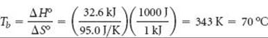
Note that we have used the conversion factor between joules and kilojoules to make the units of ΔH° and ΔS° match.

Check The experimental normal boiling point of CCl₄(l) is 76.5 °C. The small deviation of our estimate from the experimental value is due to the assumption that ΔH° and ΔS° do not change with temperature.

PRACTICE EXERCISE

Use data in Appendix C to estimate the normal boiling point, in K, for elemental bromine, Br₂(l). (The experimental value is given in Figure 11.5.)

Answer: 330 K

When the concentrations of reactants and products are nonstandard, we must calculate Q in order to determine ΔG. We illustrate how this is done in Sample Exercise 19.11. At this stage in our discussion, therefore, it becomes important to note the units used to calculate Q when using Equation 19.19. The convention used for standard states is used when applying this equation: In determining the value of Q, the concentrations of gases are always expressed as partial pressures in atmospheres and solutes are expressed as their concentrations in molarities.

SAMPLE EXERCISE 19.11 Calculating the Free-Energy Change under Nonstandard Conditions

Calculate ΔG at 298 K for a mixture of 1.0 atm N₂, 3.0 atm H₂, and 0.50 atm NH₃ being used in the Haber process:

SOLUTION

Analyze We are asked to calculate ΔG under nonstandard conditions.

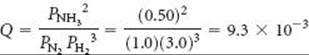
Plan We can use Equation 19.19 to calculate ΔG. Doing so requires that we calculate the value of the reaction quotient Q for the specified partial pressures, for which we use the partial-pressures form of Equation 15.23: Q = [D]^d[E]^e/[A]^a[B]^b. We then use a table of standard free energies of formation to evaluate ΔG°.

Solve The partial-pressures form of Equation 15.23 gives

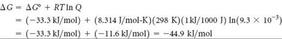
In Sample Exercise 19.9 we calculated ΔG° = –33.3 kJ for this reaction. We will have to change the units of this quantity in applying Equation 19.19, however. For the units in Equation 19.19 to work out, we will use kJ/mol as our units for ΔG°, where “per mole” means “per mole of the reaction as written.” Thus, ΔG° = –33.3 kJ/mol implies per 1 mol of N₂, per 3 mol of H₂, and per 2 mol of NH₃.

We now use Equation 19.19 to calculate ΔG for these nonstandard conditions:

Comment We see that ΔG becomes more negative as the pressures of N₂, H₂, and NH₃ are changed from 1.0 atm (standard conditions, ΔG°) to 1.0 atm, 3.0 atm, and 0.50 atm, respectively. The larger negative value for ΔG indicates a larger “driving force” to produce NH₃.

We would make the same prediction based on Le Châtelier's principle. (Section 15.7) Relative to standard conditions, we have increased the pressure of a reactant (H₂) and decreased the pressure of the product (NH₃). Le Châtelier's principle predicts that both changes shift the reaction to the product side, thereby forming more NH₃.

PRACTICE EXERCISE

Calculate ΔG at 298 K for the Haber reaction if the reaction mixture consists of 0.50 atm N₂, 0.75 atm H₂, and 2.0 atm NH₃.

Answer: –26.0 kJ/mol

Relationship Between ΔG° and K

We can now use Equation 19.19 to derive the relationship between ΔG° and the equilibrium constant, K. At equilibrium, ΔG = 0 and Q = K. Thus, at equilibrium, Equation 19.19 transforms as follows:

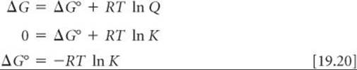
By solving Equation 19.20 for K, we obtain an expression that allows us to calculate K if we know the value of ΔG°:

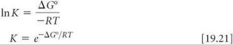
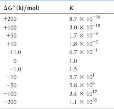
TABLE 19.4 • Relationship between ΔG° and K at 298 K

As usual, we must be careful in our choice of units. In Equations 19.20 and 19.21 we again express ΔG° in kJ/mol. In the equilibrium-constant expression, we use atmospheres for gas pressures, molarities for solutions, and solids, liquids, and solvents do not appear in the expression. (Section 15.4) Thus, the equilibrium constant is K_p for gas-phase reactions and K_c for reactions in solution. (Section 15.2)

From Equation 19.20 we see that if ΔG° is negative, ln K must be positive, which means K > 1. Therefore, the more negative ΔG° is, the larger K is. Conversely, if ΔG° is positive, ln K is negative, which means K < 1. TABLE 19.4 summarizes these relationships.

SAMPLE EXERCISE 19.12 Calculating an Equilibrium Constant from ΔG°

The standard free-energy change for the Haber process at 25 °C was obtained in Sample Exercise 19.9 for the Haber reaction:

Use this value of ΔG° to calculate the equilibrium constant for the process at 25 °C.

SOLUTION

Analyze We are asked to calculate K for a reaction, given ΔG°.

Plan We can use Equation 19.21 to calculate K.

Solve Remembering to use the absolute temperature for T in Equation 19.21 and the form of R that matches our units, we have

Comment This is a large equilibrium constant, which indicates that the product, NH₃, is greatly favored in the equilibrium mixture at 25 °C. The equilibrium constants for the Haber reaction at temperatures in the range 300 °C to 600 °C, given in Table 15.2, are much smaller than the value at 25 °C. Clearly, a low-temperature equilibrium favors the production of ammonia more than a hightemperature one. Nevertheless, the Haber process is carried out at high temperatures because the reaction is extremely slow at room temperature.

Remember Thermodynamics can tell us the direction and extent of a reaction but tells us nothing about the rate at which it will occur. If a catalyst were found that would permit the reaction to proceed at a rapid rate at room temperature, high pressures would not be needed to force the equilibrium toward NH₃.

PRACTICE EXERCISE

Use data from Appendix C to calculate ΔG° and K at 298 K for the reaction

Answer: ΔG° = –106.4kJ/mol, K = 4 × 10¹⁸

CHEMISTRY AND LIFE
DRIVING NONSPONTANEOUS REACTIONS

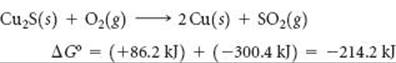
Many desirable chemical reactions, including a large number that are central to living systems, are non-spontaneous as written. For example, consider the extraction of copper metal from the mineral chalcocite, which contains Cu₂S. The decomposition of Cu₂S to its elements is nonspontaneous:

Because ΔG° is very positive, we cannot obtain Cu(s) directly via this reaction. Instead, we must find some way to “do work” on the reaction to force it to occur as we wish. We can do this by coupling the reaction to another one so that the overall reaction is spontaneous. For example, we can envision the S(s) reacting with O₂(g) to form SO₂(g):

By coupling these reactions, we can extract much of the copper metal via a spontaneous reaction:

In essence, we have used the spontaneous reaction of S(s) with O₂(g) to provide the free energy needed to extract the copper metal from the mineral.

Biological systems employ the same principle of using spontaneous reactions to drive nonspontaneous ones. Many of the biochemical reactions that are essential for the formation and maintenance of highly ordered biological structures are not spontaneous. These necessary reactions are made to occur by coupling them with spontaneous reactions that release energy. The metabolism of food is the usual source of the free energy needed to do the work of maintaining biological systems. For example, complete oxidation of the sugar glucose, C₆H₁₂O₆, to CO₂ and H₂O yields substantial free energy:

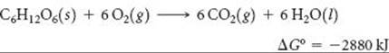
This energy can be used to drive nonspontaneous reactions in the body. However, a means is necessary to transport the energy released by glucose metabolism to the reactions that require energy. One way, shown in FIGURE 19.19, involves the interconversion of adeno-sine triphosphate (ATP) and adenosine diphosphate (ADP), molecules that are related to the building blocks of nucleic acids. The conversion of ATP to ADP releases free energy (ΔG° = –30.5kJ) that can be used to drive other reactions.

In the human body the metabolism of glucose occurs via a complex series of reactions, most of which release free energy. The free energy released during these steps is used in part to reconvert lower-energy ADP back to higher-energy ATP. Thus, the ATP-ADP interconversions are used to store energy during metabolism and to release it as needed to drive nonspontaneous reactions in the body. If you take a course in biochemistry, you will have the opportunity to learn more about the remarkable sequence of reactions used to transport free energy throughout the human body.

RELATED EXERCISES: 19.102 and 19.103

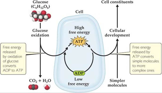
FIGURE 19.19 Schematic representation of free-energy changes during cell metabolism. The oxidation of glucose to CO₂ and H₂O produces free energy that is then used to convert ADP into the more energetic ATP. The ATP is then used, as needed, as an energy source to drive nonspontaneous reactions, such as the conversion of simple molecules into more complex cell constituents.

SAMPLE INTEGRATIVE EXERCISE Putting Concepts Together

Consider the simple salts NaCl(s) and AgCl(s). We will examine the equilibria in which these salts dissolve in water to form aqueous solutions of ions:

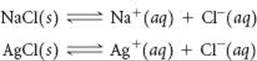
(a) Calculate the value of ΔG° at 298 K for each of the preceding reactions. (b) The two values from part (a) are very different. Is this difference primarily due to the enthalpy term or the entropy term of the standard free-energy change? (c) Use the values of ΔG° to calculate the K_sp values for the two salts at 298 K. (d) Sodium chloride is considered a soluble salt, whereas silver chloride is considered insoluble. Are these descriptions consistent with the answers to part (c)? (e) How will ΔG° for the solution process of these salts change with increasing T? What effect should this change have on the solubility of the salts?

SOLUTION

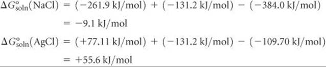
(a) We will use Equation 19.14 along with values from Appendix C to calculate the values for each equilibrium. (As we did in Section 13.1, we use the subscript “soln” to indicate that these are thermodynamic quantities for the formation of a solution.) We find

(b) We can write as the sum of an enthalpy term, , and an entropy term, . We can calculate the values of and by using Equations 5.31 and 19.8. We can then calculate . All these calculations are now familiar to us. The results are summarized in the following table:

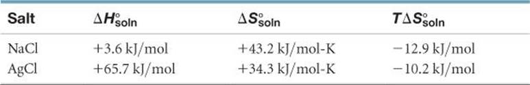
The entropy terms for the solution of the two salts are very similar. That seems sensible because each solution process should lead to a similar increase in randomness as the salt dissolves, forming hydrated ions. (Section 13.1) In contrast, we see a very large difference in the enthalpy term for the solution of the two salts. The difference in the values of is dominated by the difference in the values of .

(c) The solubility product, K_sp, is the equilibrium constant for the solution process. (Section 17.4) As such, we can relate K_sp directly to by using Equation 19.21:

We can calculate the K_sp values in the same way we applied Equation 19.21 in Sample Exercise 19.12. We use the values we obtained in part (a), remembering to convert them from kJ/mol to J/mol:

The value calculated for the K_sp of AgCl is very close to that listed in Appendix D.

(d) A soluble salt is one that dissolves appreciably in water. (Section 4.2) The K_sp value for NaCl is greater than 1, indicating that NaCl dissolves to a great extent. The K_sp value for AgCl is very small, indicating that very little dissolves in water. Silver chloride should indeed be considered an insoluble salt.

(e) As we expect, the solution process has a positive value of ΔS for both salts (see the table in part b). As such, the entropy term of the free-energy change, , is negative. If we assume that and do not change much with temperature, then an increase in T will serve to make more negative. Thus, the driving force for dissolution of the salts will increase with increasing T, and we therefore expect the solubility of the salts to increase with increasing T. In Figure 13.18 we see that the solubility of NaCl (and that of nearly any other salt) increases with increasing temperature. (Section 13.3)