CHEMISTRY THE CENTRAL SCIENCE
6 ELECTRONIC STRUCTURE OF ATOMS
6.6 REPRESENTATIONS OF ORBITALS
So far we have emphasized orbital energies, but the wave function also provides information about an electron's probable location in space. Let's examine the ways in which we can picture orbitals because their shapes help us visualize how the electron density is distributed around the nucleus.
The s Orbitals
We have already seen one representation of the lowest-energy orbital of the hydrogen atom, the 1s (Figure 6.16). The first thing we notice about the electron density for the 1s orbital is that it is spherically symmetric—in other words, the electron density at a given distance from the nucleus is the same regardless of the direction in which we proceed from the nucleus. All of the other s orbitals (2s, 3s, 4s, and so forth) are also spherically symmetric and centered on the nucleus.
Recall that the l quantum number for the s orbitals is 0; therefore, the ml quantum number must be 0. Thus, for each value of n, there is only one s orbital.
So how do s orbitals differ as the value of n changes? One way to address this question is to look at the radial probability function, also called the radial probability density, which is defined as the probability that we will find the electron at a specific distance from the nucleus.
![]() FIGURE 6.18 shows the radial probability density for the 1s, 2s, and 3s orbitals of hydrogen as a function of r, the distance from the nucleus. Three features of these graphs are noteworthy: the number of peaks, the number of points at which the probability function goes to zero (called nodes), and how spread out the distribution is, which gives a sense of the size of the orbital.
FIGURE 6.18 shows the radial probability density for the 1s, 2s, and 3s orbitals of hydrogen as a function of r, the distance from the nucleus. Three features of these graphs are noteworthy: the number of peaks, the number of points at which the probability function goes to zero (called nodes), and how spread out the distribution is, which gives a sense of the size of the orbital.
For the 1s orbital, we see that the probability rises rapidly as we move away from the nucleus, maximizing at about 0.5 Å. Thus, when the electron occupies the 1s orbital, it is most likely to be found this distance from the nucleus.* Notice also that in the 1s orbital the probability of finding the electron at a distance greater than about 3 Å from the nucleus is essentially zero.
![]() GO FIGURE
GO FIGURE
How many maxima would you expect to find in the radial probability function for the 4s orbital of the hydrogen atom? How many nodes would you expect in this function?
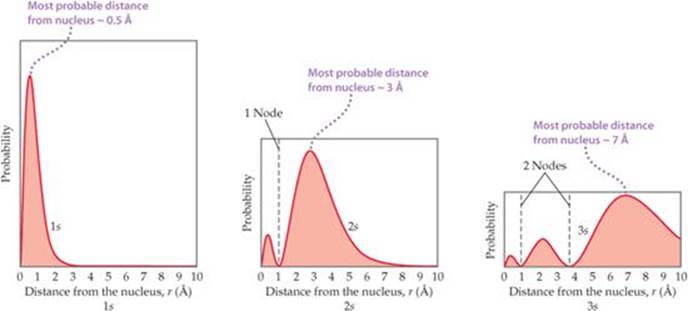
![]() FIGURE 6.18 Radial probability distributions for the 1s, 2s, and 3s orbitals of hydrogen. These graphs of the radial probability function plot probability of finding the electron as a function of distance from the nucleus. As n increases, the most likely distance at which to find the electron (the highest peak) moves farther from the nucleus.
FIGURE 6.18 Radial probability distributions for the 1s, 2s, and 3s orbitals of hydrogen. These graphs of the radial probability function plot probability of finding the electron as a function of distance from the nucleus. As n increases, the most likely distance at which to find the electron (the highest peak) moves farther from the nucleus.
Comparing the radial probability distributions for the 1s, 2s, and 3s orbitals reveals three trends:
1. The number of peaks increases with increasing n, with the outermost peak being larger than inner ones.
2. The number of nodes increases with increasing n.
3. The electron density becomes more spread out with increasing n.
One widely used method of representing orbital shape is to draw a boundary surface that encloses some substantial portion, say 90%, of the electron density for the orbital. This type of drawing is called a contour representation, and the contour representations for the s orbitals are spheres (![]() FIGURE 6.19). All the orbitals have the same shape, but they differ in size, becoming larger as n increases, reflecting the fact that the electron density becomes more spread out as n increases. Although the details of how electron density varies within a given contour representation are lost in these representations, this is not a serious disadvantage. For qualitative discussions, the most important features of orbitals are shape and relative size, which are adequately displayed by contour representations.
FIGURE 6.19). All the orbitals have the same shape, but they differ in size, becoming larger as n increases, reflecting the fact that the electron density becomes more spread out as n increases. Although the details of how electron density varies within a given contour representation are lost in these representations, this is not a serious disadvantage. For qualitative discussions, the most important features of orbitals are shape and relative size, which are adequately displayed by contour representations.
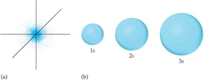
![]() FIGURE 6.19 Comparison of the 1s, 2s, and 3s orbitals. (a) Electron-density distribution of a 1s orbital. (b) Contour representions of the 1s, 2s, and 3s orbitals. Each sphere is centered on the atom's nucleus and encloses the volume in which there is a 90% probability of finding the electron.
FIGURE 6.19 Comparison of the 1s, 2s, and 3s orbitals. (a) Electron-density distribution of a 1s orbital. (b) Contour representions of the 1s, 2s, and 3s orbitals. Each sphere is centered on the atom's nucleus and encloses the volume in which there is a 90% probability of finding the electron.
 A CLOSER LOOK
PROBABILITY DENSITY AND RADIAL PROBABILITY FUNCTIONS
According to quantum mechanics, we must describe the position of the electron in the hydrogen atom in terms of probabilities. The information about the probability is contained in the wave functions, ψ, obtained from Schrödinger's equation. The square of the wave function, ψ2, called either the probability density or the electron density, as noted earlier, gives the probability that the electron is at any point in space. Because s orbitals are spherically symmetric, the value of ψ for an s electron depends only on its distance from the nucleus, r. Thus, the probability density can be written as [ψ(r)]2, where ψ(r) is the value of ψ at r. This function [ψ(r)]2 gives the probability density for any point located a distance r from the nucleus.
The radial probability function, which we used in Figure 6.18, differs from the probability density. The radial probability function equals the total probability of finding the electron at all the points at any distance r from the nucleus. In other words, to calculate this function, we need to “add up” the probability densities [ψ(r)]2 over all points located a distance r from the nucleus. FIGURE 6.20 compares the probability density at a point ([ψ(r)]2) with the radial probability function.
Let's examine the difference between probability density and radial probability function more closely. ![]() FIGURE 6.21 shows plots of [ψ(r)]2 as a function of r for the 1s, 2s, and 3s orbitals of the
FIGURE 6.21 shows plots of [ψ(r)]2 as a function of r for the 1s, 2s, and 3s orbitals of the
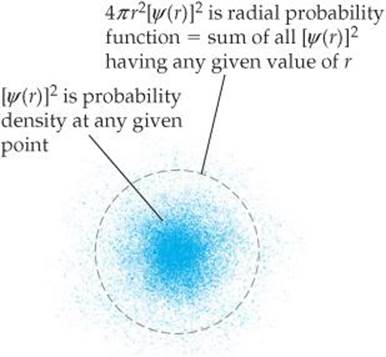
![]() FIGURE 6.20 Comparing probability density [ψ[r)]2 and radial probability function 4πr2[ψ(r)]2.
FIGURE 6.20 Comparing probability density [ψ[r)]2 and radial probability function 4πr2[ψ(r)]2.
The p Orbitals
The distribution of electron density for a 2p orbital is shown in ![]() FIGURE 6.22 (a). The electron density is not distributed spherically as in an s orbital. Instead, the density is concentrated in two regions on either side of the nucleus, separated by a node at the nucleus. We say that this dumbbell-shaped orbital has two lobes. Recall that we are making no statement of how the electron is moving within the orbital. Figure 6.22(a) portrays only the averaged distribution of the electron density in a 2p orbital.
FIGURE 6.22 (a). The electron density is not distributed spherically as in an s orbital. Instead, the density is concentrated in two regions on either side of the nucleus, separated by a node at the nucleus. We say that this dumbbell-shaped orbital has two lobes. Recall that we are making no statement of how the electron is moving within the orbital. Figure 6.22(a) portrays only the averaged distribution of the electron density in a 2p orbital.
Beginning with the n = 2 shell, each shell has three p orbitals. Recall that the I quantum number for p orbitals is 1. Therefore, the magnetic quantum number m\ can have three possible values: −1, 0, and +1. Thus, there are three 2p orbitals, three 3p orbitals, and so forth, corresponding to the three possible values of m\. Each set of p orbitals has the dumbbell shapes shown in Figure 6.22(a) for the 2p orbitals. For each value of n, the three p orbitals have the same size and shape but differ from one another in spatial orientation. We usually represent p orbitals by drawing the shape and orientation of their wave functions, as shown in Figure 6.22(b). It is convenient to label these as the px, py, and pz orbitals. The letter subscript indicates the Cartesian axis along which the orbital is oriented.* Like s orbitals, p orbitals increase in size as we move from 2p to 3p to4p, and so forth. hydrogen atom. You will notice that these plots look distinctly different from the radial probability functions shown in Figure 6.18.
As shown in Figure 6.20, the collection of points a distance r from the nucleus is the surface of a sphere of radius r. The probability density at each point on that spherical surface is [ψ(r)]2. To add up all the individual probability densities requires calculus and so is beyond the scope of this text. However, the result of that calculation tells us that the radial probability function is the probability density, [ψ(r)]2, multiplied by the surface area of the sphere, 4πr2:
Radial probability function = 4πr2[ψ(r)]2
Thus, the plots of radial probability function in Figure 6.18 are equal to the plots of [ψ(r)]2 in Figure 6.21 multiplied by 4πr2. The fact that 4πr2 increases rapidly as we move away from the nucleus makes the two sets of plots look very different from each other. For example, the plot of [ψ(r)]2 for the 3s orbital in Figure 6.21 shows that the function generally gets smaller the farther we go from the nucleus. But when we multiply by 4πr2, we see peaks that get larger and larger as we move away from the nucleus (Figure 6.18).
The radial probability functions in Figure 6.18 provide us with the more useful information because they tell us the probability of finding the electron at all points a distance r from the nucleus, not just one particular point.
RELATED EXERCISES: 6.50, 6.59, 6.60, and 6.91
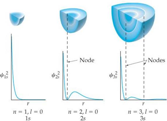
![]() FIGURE 6.21 Probability density [ψ(r)]2 in the 1s, 2s, and 3s orbitals of hydrogen.
FIGURE 6.21 Probability density [ψ(r)]2 in the 1s, 2s, and 3s orbitals of hydrogen.
![]() GO FIGURE
GO FIGURE
(a) Note on the left that the color is deep pink in the interior of each lobe but fades to pale pink at the edges. What does this change in color represent? (b) What label is applied to the 2p orbital aligned along the x axis?
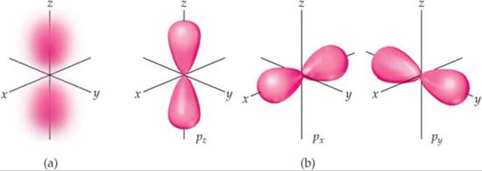
![]() FIGURE 6.22 The p orbitals.
FIGURE 6.22 The p orbitals.
(a) Electron-density distribution of a 2p orbital.
(b) Contour representations of the three p orbitals. The subscript on the orbital label indicates the axis along which the orbital lies.
The d and f Orbitals
When n is 3 or greater, we encounter the d orbitals (for which / = 2). There are five 3d orbitals, five 4d orbitals, and so forth because in each shell there are five possible values for the m\ quantum number: –2, –1, 0, 1, and 2. The different d orbitals in a given shell have different shapes and orientations in space, as shown in ![]() FIGURE 6.23. Four of the d-orbital contour representations have a “four-leaf clover” shape, and each lies primarily in a plane. The dx, y, dxz and dyz lie in the xy, xz, and yz planes, respectively, with the lobes oriented between the axes. The lobes of the dx2–y2 orbital also lie in the xy plane, but the lobes lie along the x and y axes. The dy2 orbital looks very different from the other four: It has two lobes along the z axis and a “doughnut” in the xy plane. Even though the dz2 orbital looks different from the other d orbitals, it has the same energy as the other four d orbitals. The representations in Figure 6.23 are commonly used for all d orbitals, regardless of principal quantum number. When n is 4 or greater, there are seven equivalent f orbitals (for which l = 3). The shapes of the f orbitals are even more complicated than those of the dorbitals and are not presented here. As you will see in the next section, however, you must be aware of f orbitals as we consider the electronic structure of atoms in the lower part of the periodic table.
FIGURE 6.23. Four of the d-orbital contour representations have a “four-leaf clover” shape, and each lies primarily in a plane. The dx, y, dxz and dyz lie in the xy, xz, and yz planes, respectively, with the lobes oriented between the axes. The lobes of the dx2–y2 orbital also lie in the xy plane, but the lobes lie along the x and y axes. The dy2 orbital looks very different from the other four: It has two lobes along the z axis and a “doughnut” in the xy plane. Even though the dz2 orbital looks different from the other d orbitals, it has the same energy as the other four d orbitals. The representations in Figure 6.23 are commonly used for all d orbitals, regardless of principal quantum number. When n is 4 or greater, there are seven equivalent f orbitals (for which l = 3). The shapes of the f orbitals are even more complicated than those of the dorbitals and are not presented here. As you will see in the next section, however, you must be aware of f orbitals as we consider the electronic structure of atoms in the lower part of the periodic table.
In many instances later in the text you will find that knowing the number and shapes of atomic orbitals will help you understand chemistry at the molecular level. You will therefore find it useful to memorize the shapes of the s, p, and d orbitals shown in Figures 6.19, 6.22, and 6.23.
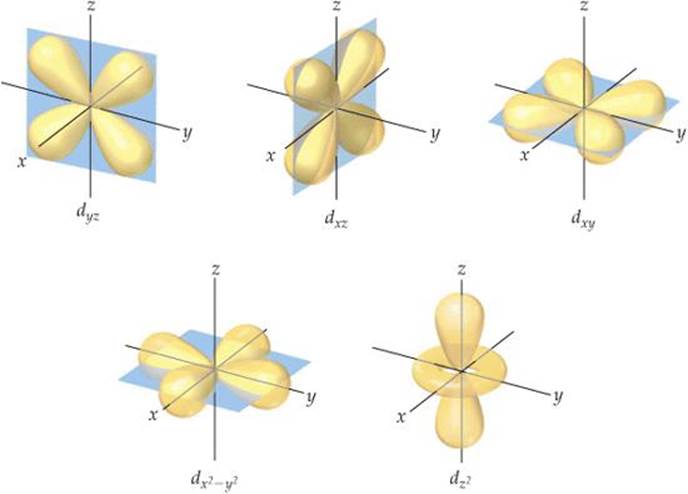
![]() FIGURE 6.23 Contour representations of the five d orbitals.
FIGURE 6.23 Contour representations of the five d orbitals.