Liquid-State Physical Chemistry: Fundamentals, Modeling, and Applications (2013)

In the theoretical description of liquids, we will encounter functions, matrices and determinants. Moreover, we will encounter scalars, vectors, and tensors. We will also need occasionally coordinate transformations, some transforms and calculus of variations. In the following we will briefly review these concepts, as well as some of the operations between them and some useful general results.

B.1 Symbols and Conventions

Often, we will use quantities with subscripts, for example, A_ij. With respect to these quantities a convenient symbol is the Kronecker delta, denoted by δ_ij and defined by

(B.1)

Note that we can write the identity Σ_iδ_ija_i = a_j, and therefore δ_ij is also called the substitution operator. Applying δ_ij to A_ij results in Σ_ijA_ijδ_ij = Σ_jA_jj.

We also introduce the alternator e_ijk for which it holds that

(B.2)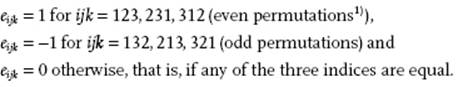

An alternative expression is given by e_ijk = ½(i − j)(j − k)(k − i).

B.2 Partial Derivatives

A function f may be dependent on variables x_i and parameters p_j, denoted by f(x_i;p_j). Reference to the parameters is often omitted by writing f(x_i). In practice, reference to the variable is also often omitted by writing just f. For a function f, several derivatives exist. If all variables but one, say x₁, are kept constant during differentiation, the derivative of f with respect to x₁ is called the partial derivative and is denoted by . Once a choice of independent variables is made, there is no need to indicate, as frequently done, which variables are kept constant. Therefore can be indicated without confusion by ∂f(x_i)/∂x₁. The function ∂f/∂x_i generally is a function of all variables x_i and, if continuous, may be differentiated again to yield the second partial derivatives ∂²f/∂x_i∂x_j (= ∂²f/∂x_j∂x_i).

Example B.1

For f(x,y) = x²y³ one simply calculates

In case the independent variables x_i increase by dx_i, the value of the function f at x_i + dx_i is given by Taylor's expansion

(B.3)

One can also write symbolically

(B.4)

Expansion of the exponential yields Eq. (B.3). Another way is to write

(B.5)

where the (nth order) differential is given by

(B.6)

Example B.2

Consider again the function f(x,y) = x²y³. A first-order estimate for f(2.1,2.1) is

using f(2,2) as the reference value. The actual value is 40.84.

A function f(x) is analytic at x = c if f(x) can be written as (a sum of) Taylor series (with a positive convergence radius). If f(x) is analytic at each point on the open interval I, f(x) is analytic on the interval I. For a function w(z) of a complex variable to be analytic, it must satisfy the Cauchy–Riemann conditions

(B.7)

where u(x,y) = Re w(z) and v(x,y) = Im w(z) denote the real and imaginary parts of w, respectively. Moreover, if u(x,y) and v(x,y) have continuous second derivatives the function w(z) obeys the Laplace equation ∂²u/∂²x + ∂²u/∂²y = ∂²v/∂²x + ∂²v/∂²y = 0, and is said to be harmonic.

Example B.3

Consider the function w(z) = e^x cos y + i e^x sin y = exp(z). Then it holds that

The derivatives are given by

Hence, Cauchy–Riemann conditions are satisfied and the function is harmonic.

B.3 Composite, Implicit, and Homogeneous Functions

If for a function f the variables x_i are themselves a function of y_j, it is called a composite function. For the first-order differentials the chain rule applies so that

(B.8)

In many cases the variables x_i are not independent, that is, a relation exists between them meaning that an arbitrary member, say x₁, can be expressed as a function of x₂, … , x_n. Often, this relation is given in the form of an implicit function, that is, f = f(x_i) = constant. Of course, if the equation can be solved, the relevant differentials can be obtained from the solution. The appropriate relations between the differentials can also be obtained by observing that df = Σ_i(∂f/∂x_i) = 0. If x₁ is the dependent variable, putting dx₁ = 0 and division by dx_i (i≠1) yields

(B.9)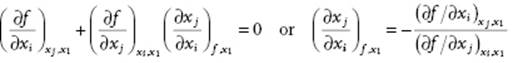

Example B.4

Consider explicitly a function f of three variables x, y and z, where z is the dependent variable. If we take x₁ = z, x_i = x and x_j = y, Eq. (B.9) reads

On the other hand, taking x_i = y and x_j = x for x₁ = z results in

Hence, it easily follows that

(B.10)

By cyclic permutation of the variables we obtain

resulting, after substitution in each other, in

(B.11)

Now consider x, y and z to be composite functions of another variable u. If f is constant, there is a relation between x, y and z and thus also between ∂x/∂u, ∂y/∂u and ∂z/∂u. Moreover, df = 0 and Eq. (B.9) explicitly reads

Further taking z as constant, independent of u, results in

Comparing with (∂y/∂x)_f,z = –(∂f/∂x)_y,z(∂f/∂y)_z,x one obtains

(B.12)

The equations, indicated by •, are frequently employed in thermodynamics.

A function f(x_i) is said to be positively homogeneous of degree n if for every value of x_i and for every λ > 0 we have

(B.13)

For such a function we have Euler's theorem

to be proven by differentiation with respect to λ first and taking λ = 1 afterwards.

Example B.5

Consider the function f(x,y) = x² + xy − y². One easily finds

Consequently, x(∂f/∂x) + y(∂f/∂y) = x(2x + y) + y(x − 2y) = 2(x² + xy − y²) = 2f. Hence, f is homogeneous of degree 2.

B.4 Extremes and Lagrange Multipliers

For obtaining an extreme of a function f(x_i) of n independent variables x_i the first variation δf has to vanish (see Section B.10). This leads to

(B.14)

and, since the variables x_i are independent and the variations δx_i are arbitrary, to ∂f/∂x_i = 0 for i = 1, …, n. If, however, the extreme of f has to be found when the x_i are dependent and satisfy r constraint functions

(B.15)

where the parameters C_j are constants, the variables x_i must also obey

(B.16)

Of course, the system can be solved in principle by solving Eq. (B.15) for the independent n − r variables x_i as functions of the others, but the procedure is often complex. It can be shown that finding the extreme of f subject to the constraint of Eq. (B.15) is equivalent to finding the extreme of a function g defined by

(B.17)

where now the original variables x_i and the additional variables λ_j, called the Lagrange (undetermined) multipliers, are to be considered independent. Variation of λ_j leads to Eq. (B.15) and variation of x_i to

(B.18)

From Eq. (B.18) the values for x_i can be determined. These values are still functions of λ_j but they can be eliminated using Eq. (B.15). In physics, chem­­istry and materials science, the Lagrange multiplier often can be physically interpreted.

Example B.6

One can ask what is the minimum circumference L of a rectangle given the area A. Denoting the edges by x and y, the circumference is given by L = 2(x + y), while the area is given by A = xy. The equations to be solved are

Hence, the solution is x = y, and .

B.5 Legendre Transforms

In many problems we meet the demand to interchange between dependent and independent variables. If f(x_i) denotes a function of n variables x_i, we have

(B.19)

Elimination of x_i from X_i(x_i) and f(x_i) leads to f = f(X_i). However, from f(X_i) it is impossible to uniquely recover f(x_i) by repeating this procedure for f(X_i). Now consider the function g = f − X₁x₁. For the differential we obtain

(B.20)

and we see that the roles of x₁ and X₁ have been interchanged. This transformation can be applied to only one variable, to several variables or to all variables. In the last case we use g = f − Σ_iX_ix_i and obtain dg = –Σ_jx_jdX_j (j = 1, … ,n). This so-called Legendre transformation, if applied to the transform, results in the complete original expression and is often used in thermodynamics. For example, the Gibbs energy G(T,P) with pressure P and temperature T as independent variables results from the internal energy U(S,V) with entropy S and volume V as independent variables using G = U − TS + PV.

Example B.7

Consider the function f(x) = ½x². The dependent variable X is given by

which can be solved to yield x = X. Therefore, the function expressed in the variable X reads f(X) = ½X². For the transform g(X) one thus obtains

B.6 Matrices and Determinants

A matrix is an array of numbers (or functions), represented by a roman boldface uppercase symbol, for example, A, or by an italic uppercase symbol with indices, for example, A_ij. In full we write

(B.21)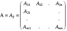

The numbers A_ij are called the elements. The matrix with m rows and n columns is called an m×n matrix or a matrix of order (m,n). The transpose of a matrix, indicated by a superscript T, is formed by interchanging rows and columns. Hence

(B.22)

Often, we will use square matrices A_ij for which m = n (order n). A column matrix (or column for short) is a matrix for which n = 1 and is denoted by a lowercase italic standard symbol with an index, for example, by a_i, or by a lowercase roman bold symbol, for example, a. A row matrix is a matrix for which m = 1 and is the transpose of a column matrix and thus denoted by (a_i)^T or a^T.

Two matrices of the same order are equal if all their corresponding elements are equal. The sum of two matrices A and B of the same order is given by the matrix C whose corresponding elements are the sums of the elements of Aand B or

(B.23)

The product of two matrices A and B results in matrix C whose elements are given by

(B.24)

representing the row-into-column rule. Note that, if A represents a matrix of order (k,l) and B a matrix of order (m,n), the product BA is not defined unless k = n. For square matrices, we generally have AB ≠ BA, so that the order must be maintained in any multiplication process. The transpose of a product (ABC..)^T is given by (ABC..)^T = ..^TC^TB^TA^T.

A real matrix is a matrix with real elements only while a complex matrix is a matrix with complex elements. The complex conjugate of a matrix A is the matrix A* formed by the complex conjugate elements of A or

(B.25)

If a real (complex), square matrix A is equal to its transpose (complex conjugate)

(B.26)

then A is a symmetric (Hermitian) matrix. For an antisymmetric matrix it holds that

(B.27)

and thus A has the form

(B.28)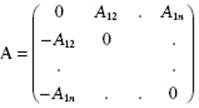

A diagonal matrix has only non-zero entries along the diagonal:

(B.29)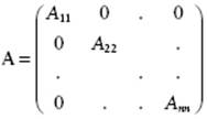

The unit matrix I is a diagonal matrix with unit elements:

(B.30)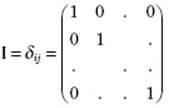

Obviously, IA = AI = A, where A is any square matrix of the same order as the unit matrix.

The determinant of a square matrix of order n is defined by

(B.31)

where the summation is over all permutations of the indices i, j, k, ···, p. The sign in brackets is positive (negative) when the permutation involves an even (odd) number of permutations from the initial term A₁₁A₂₂A₃₃..A_nn.

Example B.8

For a matrix A of order 3, Eq. (B.31) yields

Alternatively, it can be written as det A = Σ_r,s,t e_rst A_1r A_2s A_3t.

The determinant of the product AB is given by

(B.32)

Further, the determinant of a matrix equals the determinant of its transpose, that is

(B.33)

The inverse of a square matrix A is denoted by A⁻¹ and it holds that

(B.34)

where I is the unit matrix of the same order as A. Hence, a square matrix commutes with its inverse. The inverse only exists if det A ≠ 0. The inverse of the product (ABC..)⁻¹ is given by (ABC..)⁻¹ = ..⁻¹C⁻¹B⁻¹A⁻¹. The inverse of a transpose is equal to the transpose of the inverse, that is, (A^T)⁻¹ = (A⁻¹)^T, often written as A^−T.

The cofactor α_ij of the element A_ij is (–1)^i+j times the minor θ_ij. The latter is the determinant of a matrix obtained by removing row i and column j from the original matrix. The inverse of A is then found from Cramers' rule

(B.35)

Note the reversal of the element and cofactor indices.

Example B.9

Consider the matrix . The determinant is det A = –2. The cofactors are given by

The elements of the inverse A⁻¹ are thus given by

For a diagonal matrix A the inverse is particularly simple and given by

(B.36)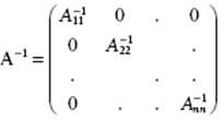

For an orthogonal (unitary) matrix it holds that

(B.37)

implying det A = ±1. With det A = 1, the matrix A is a proper orthogonal matrix.

B.7 Change of Variables

It is also often required to use different independent variables, in particular in integrals. For definiteness consider the case of three “old” variables x, y and z and three “new” variables u, v and w. In this case, we have

where the functions u, v and w are continuous and have continuous first derivatives in some region R*. The transformations u(x,y,z), v(x,y,z) and w(x,y,z) are such that a point (x,y,z) corresponding to (u,v,w) in R* lies in a region R and that there is a one-to-one correspondence between the points (u,v,w) and (x,y,z). The Jacobian matrix J = ∂(x,y,z)/∂(u,v,w) is defined by

(B.38)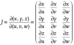

The determinant, det J, should be either positive or negative throughout the region R*. Consider now the integral

(B.39)

over the region R. If the function F is now expressed in u, v and w instead of x, y and z, the integral has to be evaluated over the region R* as

(B.40)

where |det J| denotes the absolute value of the determinant of the Jacobian matrix²⁾ J. The expression is easily generalized to more variables than 3.

Example B.10

In many cases the use of cylindrical coordinates is convenient. Here, we consider the Cartesian coordinates x₁, x₂ and x₃ as “new” variables and the cylindrical coordinates r, θ and z as “old” variables. The relations between the Cartesian coordinates and the cylindrical coordinates (Figure B.1) are

while the inverse equations are given by

Figure B.1 (a) Cylindrical and (b) spherical coordinates.

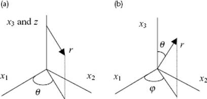
The Jacobian determinant is easily calculated as |det J| = r. Similarly, for spherical coordinates³⁾

and the corresponding inverse equations

In this case the Jacobian determinant becomes |det J| = r² sin θ.

B.8 Scalars, Vectors, and Tensors

A scalar is an entity with a magnitude. It is denoted by an italic, lowercase or uppercase, roman or greek letter, for example, a, A, γ, or Γ.

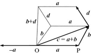
A vector is an entity with a magnitude and direction. It is denoted by a lowercase boldface, italic letter, for example, a. It can be interpreted as an arrow from a point O (origin) to a point P. Let a be this arrow. Its magnitude(length), equal to the distance OP, is denoted by a = |a|. A unit vector in the same direction as the vector a, here denoted by e, has a length of 1. Vectors obey the following rules (Figure B.2):

· c = a + b = b + a (commutative rule)

· a + (b + d) = (a + b) + d (associative rule)

· (a + b)·c = a·c + b·c (distributive law)

· a + (−a) = 0 (zero vector definition)

· a = |a|e, |e| = 1 (unit vector definition)

· 0·u = 0

· αa = α|a|e, |e| = 1

Figure B.2 Vector properties.

Various products can be formed using vectors. The scalar (or dot or inner) product of two vectors a and b yields a scalar and is defined as a·b = b·a = |a| |b|cos(ϕ), where ϕ is the enclosed angle between a and b. From this definition it follows that a = |a| = (a·a)^1/2. Two vectors a and b are orthogonal if a·b = 0. The scalar product is commutative (a·b = b·a) and distributive (a·(b + c) = a·b + a·c).

The vector (or cross or outer) product of a and b denotes a vector c = a × b. We define a unit vector n perpendicular to the plane spanned by a and b. The sense of n is right-handed: rotate from a to b along the smallest angle and the direction of n is given by a right-hand screw. It holds that a·n = b·n = 0 and |n| = 1. Explicitly, n = a × b/|a| |b|. The vector product c is equal to c = a × b = −b × a = |a| |b|sin(ϕ)n. The length of |c| = |a| |b|sin(ϕ) is numerically equal to the area of the parallelogram whose sides are given by a and b. The vector product is anti-commutative (a × b = −b × a) and distributive (a × (b + c) = a × b + a × c), but not associative (a × (b × c) ≠ (a × b) × c).

The triple product is a scalar and given by d = a·b × c = a × b·c. It yields the volume of the block (or parallelepepid) the edges of which are a, b, and c. Three vectors a, b, and c are independent if from αa + βb + γc = 0 it follows that α = β = γ = 0. This is only the case if a, b and c are noncoplanar or, equivalently, the product a·b × c ≠ 0.

Finally, we need the tensor (or dyadic) product ab. Operating on a vector c, it associates with c a new vector according to ab·c = a(b·c) = (b·c)a. Note that ba operating on c yields ba·c = b(a·c) = (a·c)b.

A tensor (of rank 2), denoted by an uppercase boldface, italic letter, for example, A, is a linear mapping that associates with a vector a another vector b according to b = A·a. Tensors obey the following rules:

· C = A + B = B + A (commutative law)

· A + (B + C) = (A + B) + C (associative law)

· (A + B)·u = A ·u + B·u (distributive law)

· A + (−A) = O (zero tensor definition)

· I·u = u (I unit tensor definition)

· O·u = 0 (O zero tensor, 0 zero vector)

· A ·(αu) = (αA)·u = α(A·u)

where α is an arbitrary scalar and u is an arbitrary vector. The simplest example of a tensor is the tensor product of two vectors, for example, if A = bc, the vector associated with a is given by A·a = bc·a = (c·a)b.

So far we have discussed vectors and tensors using the direct notation only, that is using a symbolism, which represents the quantity without referring to a coordinate system. It is convenient though to introduce a coordinate system. In this book we will make use primarily of Cartesian coordinates, which are a rectangular and rectilinear coordinate system with origin O and unit vectors e₁, e₂ and e₃ along the axes. The set e_i = {e₁, e₂, e₃} is called an orthonormal basis. It holds that e_ie_j = δ_ij. The vector OP = x is called the position of point P. The real numbers x₁, x₂ and x₃, defined uniquely by the relation x = x₁e₁ + x₂e₂ + x₃e₃, are called the (Cartesian) components of the vector x. It follows that x_i = x·e_i for i = 1, 2, 3. Using the components x_i in equations, we use the index notation. Using the index notation the scalar product u·v can be written as u·v = u₁v₁ + u₂v₂ + u₃v₃ = Σ_iu_iv_i. The length of a vector x, |x| = (x·x)^1/2, is thus also equal to . Sometimes, it is also convenient to use matrix notation; in this case the components x_i are written collectively as a column matrix x. In matrix notation the scalar product u·v is written as u^Tv. The tensor product ab in matrix notation is given by ab^T.

Using the alternator e_ijk the relations between the unit vectors can be written as e_i×e_j = Σ_ke_ijke_k. Similarly, the vector product c = a × b can alternatively be written as c = a × b = Σ_j,k e_ijke_ia_jb_k. In components this leads to the following expressions:

(B.41)

The triple product a·b × c in components is given by e_ijka_ib_jc_k, while the tensor product ab is represented by a_ib_j. A useful relation involving three vectors using the tensor product is a × (b × c) = (ba − (a·b)I)·c.

If e_i = {e₁, e₂, e₃} is a basis, the tensor products e_ie_j, i, j = 1, 2, 3, form a basis for representing a tensor, and we can write A = A_kle_ke_l. The nine real numbers A_kl are the (Cartesian) components of the tensor A, and are conveniently arranged in a square matrix. It follows that A_kl = e_k·(A·e_l), which can be taken as the definition of the components. Applying this definition to the unit tensor, it follows that δ_kl are the components of the unit tensor, that is, I = δ_kle_ke_l. If v = A·u, we also have v = (A_kle_ke_l)·u = e_kA_klu_l. Tensors, like vectors, can form different products. The inner product A·B of two tensors (of rank 2) A and B yields another tensor of rank 2 and is defined by (A·B)·u = A·(B·u) = Σ_p,mA_kpB_pmu_m wherefrom it follows that (A·B)_km = Σ_pA_kpB_pm, representing conventional matrix multiplication. The expression A:B denotes the double inner product, yields a scalar and is given in index notation by Σ_i,jA_ijB_ij. Equivalently, A:B = tr AB^T = tr A^TB.

Recall that the components of a vector a can be transformed to another Cartesian frame by in index notation, or a′ = Ca in matrix notation. Since a tensor A of rank 2 can be interpreted as the tensor product of two vectors b and c, that is,

the transformation rule for the components of a tensor A obviously is

or, in matrix notation⁴⁾

If A′ = A and thus A′ = A, then A is an isotropic (or spherical) tensor. Further, if the component matrix of a tensor has a property which is not changed by a coordinate axes rotation that property is shared by A′ and A. Such a property is called an invariant. An example is the transpose of a tensor of rank 2: If A′ = CAC^T, then A′^T = CA^TC^T. Consequently, we may speak of the transpose A^T of the tensor A, and we may define the symmetric parts A^(s) and antisymmetric A^(a) parts by

While originally a distinction in terminology is made for a scalar, a vector and a tensor, it is clear that they all transform similarly under a coordinate transformation. Therefore, a scalar is sometimes denoted as a tensor of rank 0 and a vector as a tensor of rank 1. Expressed in components, all tensors obey the same type of transformation rules, for example, A_i…j = Σ_p,…,qC_ip …C_jq A_p…q, where the transformation matrix C represents the rotation of the coordinate system. Scalars have no index, a vector has one index, a tensor of rank 2 has two indices, while a tensor of rank 4 has four indices. Their total transformation matrix contains a product of respectively 0, 1, 2, and 4 individual transformation matrices C_ij. Obviously, if we define (Cartesian) tensors as quantities obeying the above transformation rules⁵⁾, extension to any order is immediate.

Finally, we have to mention that, like scalars, vectors and tensors can be a function of one or more variables x_k. The appropriate notation is f(x_k), a_i(x_k) and A_ij(x_k) or, equivalently, f(x), a(x) and A(x). If x_k represent the coordinates, f(x), a(x) and A(x) are referred to as a scalar, vector, and tensor field, respectively.

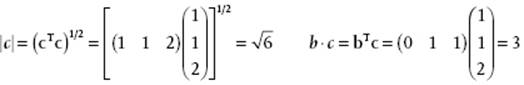
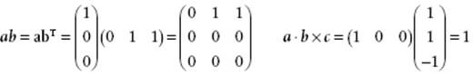
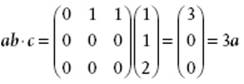
Example B.11

Consider the vectors a, b and c the matrix representations of which are

B.9 Tensor Analysis

In this section we consider various differential operators, the divergence and some other theorems and their representation in cylindrical and spherical coordinates. Consider a_i as a typical representative of tensors of rank 1 and take the partial derivatives ∂a_i/∂x_j. Such a derivative transforms like a tensor of rank 2, is called the gradient and is denoted by grad a_i in index notation or as ∇a in direct notation. The gradient can operate on any tensor thereby increasing its rank by 1.

Summing over an index, known as contraction, decreases the rank of a tensor by 2. If we apply contraction to a tensor A_ij we calculate Σ_iA_ii and the result is known as the trace, written in direct notation as tr A. Contraction of a gradient Σ_i(∂a_i/∂x_i) yields a scalar, called divergence and denoted in direct notation by div a or ∇·a.

Another operator is the curl (or rot as abbreviation of rotation) of a vector a, in direct notation written as ∇ × a, which is a vector with components ∂_k,je_ijk∂a_k/∂x_j. It is defined for 3D space only.

Finally, we have the Laplace operator. This can act on a scalar a or on a vector a, is denoted by ∇² or Δ, and is defined by ∇²a = Δa = ∂a²/∂²x_i or ∇²a = Δa = ∂a_j²/∂²x_i.

Example B.12

If a vector field a(x) represented by a^T(x) = (3x² + 2y, x + z², x + y²), then

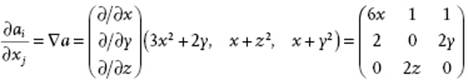
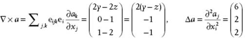
and .

Introducing now some general theorems, let us first recall that if X = ∇x with x a scalar, we have

(B.42)

Second, without proof we introduce the divergence theorem. Therefore, we consider a region of volume V with a piecewise smooth surface S on which a single-valued tensor field A or A_ij is defined. The body may be either convex or nonconvex. The components of the exterior normal vector n of S are denoted by n_i. The divergence theorem or the theorem of Gauss states that

(B.43)

The divergence theorem connects a volume integral (integrating over dV) to a surface integral (integrating over ndS) and is mainly used in theoretical work. Applying the divergence theorem to a scalar a, a vector a or a tensor Σ_k,jε_ijk∂a_k/∂x_j we obtain in direct notation

(B.44)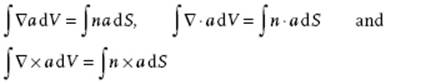

Third, one can also derive Stokes' theorem

(B.45)

The theorem connects a surface (integrating over ndS) and line integral (integrating over dr) and implies that the surface integral is the same for all surfaces bounded by the same curve. By the way, the surface element ndS is also often written as dS.

From Eq. (B.42), (B.43) and (B.45) one can derive many transformations of integrals. We only mention Green's first identity (using ndS = dS)

(B.46)

and Green's second identity

(B.47)

The above operations can also be performed in other coordinate systems. Often, one considers systems where the base vectors locally still form an orthogonal basis, although the orientation may differ through space. These systems are normally addressed as orthogonal curvilinear coordinates. Cylindrical and spherical coordinates form examples with practical importance. Using the relations of Example B.10 one can show that the unit vectors for cylindrical coordinates are

so that the only non-zero derivatives are

Using the chain rule for partial derivatives, one may show that the gradient becomes

(B.48)

The divergence of a vector a becomes

(B.49)

while the Laplace operator acting on a scalar a is expressed by

(B.50)

Using again the relations of Example B.10, one can show that the unit vectors for spherical coordinates are

so that the only non-zero derivatives are

The gradient operator becomes

(B.51)

The divergence of a vector a becomes

(B.52)

while the Laplace operator acting on a scalar a is expressed by

(B.53)

B.10 Calculus of Variations

One of the chief applications of the calculus of variations is to find a function for which some given integral has an extreme. We treat the problem essentially as one-dimensional, but extension to more than one dimension is straightforward.

Suppose we wish to find a path x = x(t) between two given values x(t₁) and x(t₂) such that the functional⁶⁾ of some function with is an extremum. Let us assume that x₀(t) is the solution we are looking for. Other possible curves close to x₀(t) are written as x(t,α) = x₀(t) + αη(t), where η(t) is any function that satisfies η(t₁) = η(t₂) = 0. Using such a representation, the integral J becomes a function of α,

(B.54)

and the condition for obtaining the extremum is (dJ/dα)_α=0 = 0. We obtain

(B.55)

Through integration by parts the second term of the integral evaluates to

(B.56)

At t₁ and t₂, η(t) = ∂x/∂α vanishes and we obtain for Eq. (B.55)

If we define the variations δJ = (dJ/dα)_α=0dα and δx = (dx/dα)_α=0dα, we find

(B.57)

and since η must be arbitrary

(B.58)

Once this so-called Euler condition is fulfilled an extremum is obtained. It should be noted that this extremum is not necessarily a minimum. Finally, we note that in case the variations at the boundaries do not vanish, that is, the values of η are not prescribed, the boundary term evaluates, instead of to zero, to

(B.59)

If we now require δJ = 0 we obtain in addition to Eq. (B.58) also the boundary condition at t = t₁ and t = t₂.

Example B.13

Let us calculate the shortest distance between two points in a plane. An element of an arc length in a plane is

and the total length of any curve between two points 1 and 2 is

The condition that the curve is the shortest path is

Since and , we have or , wherec is a constant. This solution holds if where a is given by a = c/(1 + c²)^1/2. Obviously, this is the equation for a straight line y = ax + b, where b is another constant of integration. The constants aand b are determined by the condition that the curve should go through (x₁,y₁) and (x₂,y₂).

B.11 Gamma Function

The gamma function is defined by

For this function it generally holds that Γ(t + 1) = tΓ(t). For integer n it is connected to the more familiar factorial function n! by Γ(n + 1) = n! = n(n − 1)(n − 2)···(2)(1). Using x = y², we obtain

which results by setting t = ½ in . Consequently,

B.12 Dirac and Heaviside Function

The Dirac (delta) function δ (x) is in one dimension defined by

(B.60)

where a > 0 and a = ∞ is included and which selects the value of a function f at the value of variable t from an integral expression. Alternatively, δ (x) is defined by

(B.61)

Some properties of the delta function for a > 0 are

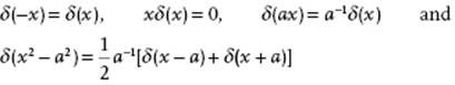
The derivative⁷⁾ δ′(x) is related to f′(x) as follows

This leads further to

Related is the Heaviside (step) function h(x), defined by

(B.62)

For a, b > 0 we have

so that the step function can be considered as the integral of the delta function.

B.13 Laplace and Fourier Transforms

The Laplace transform of a function f(t), defined by

(B.63)

transforms f(t) into where s may be real or complex. The operation is linear, that is,

The convolution theorem states that the product of two Laplace transforms L[f(t)] and L[g(t)] equals the transform of the convolution of the functions f(t) and g(t)

(B.64)

Since the Laplace transform has the property

it can transform differential equations in t to algebraic equations in s. Generalization to higher derivatives is straightforward and reads

Similarly, for integration it is found that

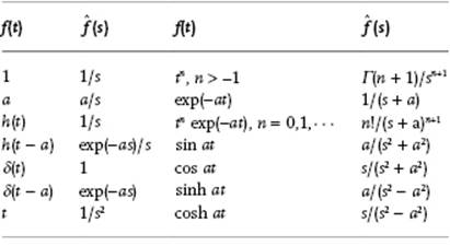
Some useful transforms are given in Table B.1.

Table B.1 Laplace transform pairs.

The Fourier transform of a function f(t) and its inverse are defined by

(B.65)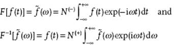

The normalization constants N^(–) and N⁽⁺⁾ can take any value as long as their product is (2π)⁻¹. If N^(–) = N⁽⁺⁾ = (2π)^−1/2 is taken, the transform is called symmetric. The Fourier transform is a linear operation for which the convolution theorem holds.

Since for the delta function δ(t) it holds that

we have as a representation of the delta function

Using

we can represent δ(t) as

Similarly, for the 3D delta function δ(t) for a vector t we have

Finally, we note that by the Gauss theorem applied to a sphere with radius r

since ∇²(1/r) = 0 for r ≠ 0 and ∇²(1/r) = ∞ for r = 0. Therefore, we have

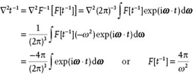
Applying the inverse transform we obtain or

B.14 Some Useful Integrals and Expansions

Several integrals and expansions, given without further comment, are useful throughout.

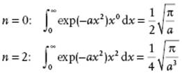
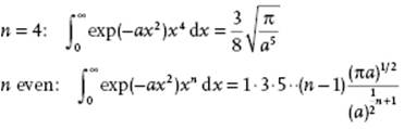
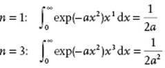
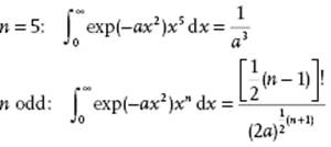
Integrals

Bi- and Multinomial Expansion

Sine Cosine and Tangent

Exponential and Logarithm

Reversion of series

Euler McLaurin formula

Denoting the derivative dⁿf(x)/dxⁿ|_x=a by f_n(a), the Euler–McLaurin expression reads

with Bernoulli numbers B₁ = 1/6, B₂ = 1/30, B₃ = 1/42, B₄ = 1/30, … .

Notes

1) An even (odd) permutation is the result of an even (odd) number of binary interchanges. The character (even or odd) of a permutation is independent of the order of the binary interchanges.

2) In the literature the name Jacobian sometimes indicates the Jacobian determinant instead of the matrix of derivatives. To avoid confusion, we use Jacobian matrix and Jacobian determinant explicitly.

3) Unfortunately in the usual convention for spherical coordinates the angle φ corresponds to the angle θ in cylindrical coordinates.

4) Obviously if the transformation is interpreted as a rotation of the tensor instead of the frame, we obtain A′ = C^TAC. This is the conventional definition of an orthogonal transformation.

5) This transformation rule is only appropriate for proper rotations of the axes. For improper rotations, which involve a reflection and change of handedness of the coordinate system, there are two possibilities. If the rule applies we call the tensor polar; if an additional change of sign occurs for an improper rotation we call the tensor axial. Hence, generally L_i..j = (det C)^p C_ik…C_jlL_k..l, where p = 0 for a polar tensor and p = 1 for an axial tensor. Since det C = 1 for a proper rotation and det C = –1 for an improper rotation, this results in an extra change of sign for an axial tensor under improper rotation. It follows that the inner and outer product of two polar or two axial tensors is polar, while the product of a polar and an axial tensor is axial. The permutation tensor e_ijk is axial since e₁₂₃ = 1 for both right-handed and left-handed systems. Hence, the vector product of two polar vectors is axial. If one restricts oneself to right-handed systems, the distinction is irrelevant.

6) A function maps a number on a number. A functional maps a function on a number.

7) A prime denotes differentiation with respect to its argument.

Further Reading

Adams, R.A. (1995) Calculus, 3rd edn, Addison-Wesley, Don Mills, ON.

Jeffreys, H. and Jeffreys, B.S. (1972) Methods of Mathematical Physics, Cambridge University Press, Cambridge.

Kreyszig, E. (1988) Advanced Engineering Mathematics, 6th edn, John Wiley & Sons, Inc., New York.

Margenau, H. and Murphy, G.M. (1956) The Mathematics of Physics and Chemistry, 2nd edn, van Nostrand, Princeton, NJ.