Liquid-State Physical Chemistry: Fundamentals, Modeling, and Applications (2013)

3.2. Electrostatic Interaction

The Coulomb energy w of a charge q₁ in the presence of another charge q₂ is

(3.4)

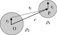
Here, ϕ₂ represents the potential associated with the force between the charges q₁ and q₂ with r = |r| their distance and ε₀ the permittivity of vacuum. Molecule 1 can be represented by a charge distribution⁴⁾ , and the potential ϕ₂ due to the charge distribution of molecule 2 by where s_j = |s_j| = |r−r_j| is the distance of charge q_j to position r (Figure 3.2). The total interaction energy with s_jk = |s_jk| = |r_j − r_k|. After expanding the function ϕ₂, evaluating all the derivatives and collecting terms, a procedure with considerable understatement often called “a lengthy but straightforward calculation” (see Justification 3.1), one obtains the desired result. Note that, since this process takes place at constant T and V, the interaction W₁₂ represents the Helmholtz energy.

Figure 3.2 The interaction ρ₁ϕ₂ of two charge distributions ρ₁ and ρ₂ with common origin O.

Justification 3.1: The multipole expansion*

To find the proper expression for the electrostatic interaction, let us consider an arbitrary charge distribution ρ of point charges q_j at position r_j from the origin O located at the center of mass (Figure 3.2). The potential energy ϕ at a certain point P located at r outside the sphere containing all charges is

where s_j = |s_j| = |r−r_j| is the distance of charge q_j to P. Developing 1/s_j in a Taylor series with respect to r_j, we may write 1/s_j = 1/r + r_j(∇1/r)_O + ··· and therefore (using direct notation, Appendix B)

(3.5)

where r = |r| is the distance of the point P to the origin O of ρ. In the second line we defined q = Σ_jq_j as the total charge, μ = Σ_jq_jr_j as the dipole moment, and Q = ½Σ_jq_jr_jr_j as the quadrupole moment. Moreover, we abbreviate 1/r by ϕ(0), [∇(1/r)]_O by φ′(0), etc. The minus sign in the last step for the second, fourth, and so on terms arises because the differentiation is now made at P, and not at the origin of the potential O. This follows since for an arbitrary vector x it holds that ∇(1/x) = −x/x³ and therefore [∇(1/r)]_P = −[∇(1/r)]_O. Equation (3.5) is usually called the multipole expansion of the potential. The interaction W of a point charge q at r in the potential ϕ of a charge distribution is W = qϕ(r). Hence, to calculate the interaction energy between two charge distributions ρ₁ and ρ₂, separated by r (Figure 3.2), we express this energy as the energy of in the field of . The interaction energy W₁₂ = ρ₁ϕ₂ is then

If we take the center of mass P of ρ₁ as common origin, the potential ϕ₂ due to ρ₂ is given by the last line of Eq. (3.5), and substitution in the previous equation results in

(3.6)

This is the general expression for the electrostatic interaction energy expressed in terms of multipole moments of the charge distributions with respect to their own center of mass [1]. For further evaluation, we need again ∇(1/r) = −r/r³ and also ∇²(1/r) = 3rr/r⁵ – I/r³ with I the unit tensor, easily derived using r² = x² + y² + z², and leading to Eq. (3.7).

The final result reads

(3.7)

or explicitly (see Figure 3.3 for notation, introducing the abbreviation ω = θ,ϕ)

(3.8)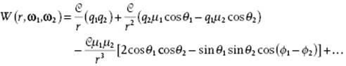

Figure 3.3 The interaction at a distance r of a point charge q₁ with a dipole μ₂ in which the charges q are separated by a distance δ (a) and the interaction of a dipole with a dipole at distance r (b).

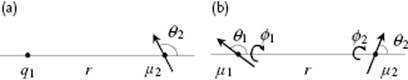
In this expression is the charge of molecule 1, and is the dipole moment with μ₁ = |μ₁|.

The first term (proportional to q₁, q₂ and 1/r) is just the Coulomb interaction (more precisely the charge–charge Coulomb interaction) between the molecules at distance r. At long distance r this interaction term will dominate, but clearly it is zero if one of the molecules is neutral.

The second term (proportional to q₁, μ₂, q₂, μ₁ and 1/r²; Figure 3.3) is the interaction between the charge of molecule 2 with the dipole moment of molecule 1 and the interaction between the charge of molecule 1 with the dipole moment of molecule 2. This is the charge–dipole (Coulomb) interaction. The charge–dipole interaction decreases as 1/r², as compared to 1/r for the charge–charge Coulomb interaction. A simple way to obtain this result is dealt with in Problem 3.2. Because the charge–dipole interaction is orientation-dependent and molecules move generally rather rapidly, an orientational average (overbar) must be made (we will learn how to do that in Chapter 5). For the moment we just quote the result, valid for sufficiently high temperature,

(3.9)

The third term (proportional to μ₁, μ₂ and 1/r³; Figure 3.3) represents the dipole–dipole (Coulomb) interaction between the dipole moments of molecule 1 and molecule 2, and is often addressed as the Keesom interaction (it also includes the charge–quadrupole interaction, but we neglect that interaction). We deal with this interaction in a simplified way in Problem 3.3. This interaction is also orientation-dependent and for the orientational average one obtains, again for sufficiently high temperature and using ω = (θ,ϕ) with θ and ϕ the orientation angles

(3.10)

For neutral molecules the dipole–dipole interaction is the leading term. Note (again) that the expressions given represent the Helmholtz energies and that the internal energy expressions U are given by U = 2W (see Problem 2.6).

Problem 3.1

Show that for a charged molecule the dipole moment depends on the choice of the origin but is independent of this choice for a neutral molecule.

Problem 3.2: Charge–dipole interaction

A simple model to estimate the charge–dipole interaction is shown in Figure 3.3. The distances between the charge q₁ of molecule 1 and the charges of the dipole moment of molecule 2, +q₂ and −q₂, respectively, are given by

Show, if it is assumed that the distance r is much larger than the distance δ by using Coulomb's law and the binomial expansion, that the interaction for fixed direction is where . How large should r be as compared to δ in order to have an error less than 5%?

Problem 3.3: Dipole–dipole interaction

The dipole–dipole interaction can be estimated in a similar way as for the charge–dipole problem (Figure 3.3). Show that the expression for the in-line orientation energy (orientations parallel to the connection line) is

Here, ± indicates whether the orientation is in the same way (attraction) or in the opposite way (repulsion). Also show that the expression for the parallel orientation energy (orientations perpendicular to the connection line) is

again, dependent on whether the orientation is antiparallel (attraction) or parallel (repulsion). How large should r be as compared to δ in order to have an error less than 5%?

Problem 3.4*

Verify Equation (3.6). Alternatively, derive the expression for the electrostatic interaction up to second order using a double Taylor expansion for with s_ij = |r + r_j−r_i| using the complete expression .