Liquid-State Physical Chemistry: Fundamentals, Modeling, and Applications (2013)

6.2. The Meaning of Structure for Liquids

Because the positions of molecules in liquids are neither regular nor completely random, we are forced to use a statistical description of their whereabouts. Therefore, the distribution function approach can be used to describe the structure of liquids.

6.2.1 Distributions Functions

Suppose that we want to know the distribution of specific molecules at specific positions. We denote the specific distribution function of N molecules by n^(N). As an example, assume that the distribution function n⁽³⁾ for three particles is given, and that n⁽²⁾ is to be determined. Now, since n⁽³⁾ = n⁽³⁾(r₁,r₂,r₃), where the independent (Cartesian) coordinates of particle i have been indicated by r_i, we obtain

This type of relation is generally valid and leads to

(6.1)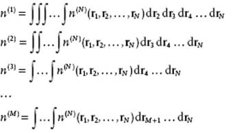

However, molecules are indistinguishable and we should ask for the generic distribution functions ρ^(N), describing any molecule at specific positions. Let us take the same example and determine ρ⁽²⁾, assuming that the distribution function n⁽³⁾ for three particles is given. In this case we have ρ⁽³⁾ = 3 × 2 × 1 n⁽³⁾(r₁,r₂,r₃) = 3! n⁽³⁾(r₁,r₂,r₃). Further, we obtain

These relations can also be generalized for N particles, and we obtain

(6.2)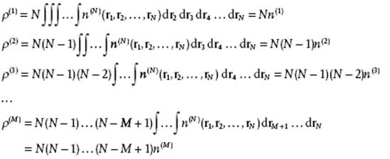

Equivalently, we can write N(N − 1) … (N − M + 1) = N!/(N − M)!. Hence, generally,

(6.3)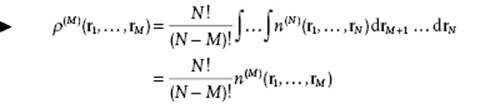

From this expression we can also easily derive that

(6.4)

(6.5)

Extending these ideas, from position coordinates r to position coordinates r plus momenta p, results in

(6.6)

where, as before, r = (r₁,r₂, … ,r_N) and p = (p₁,p₂, … ,p_N). This function describes the probability of M molecules to be at positions r meanwhile having momenta p.

The simplest distribution function ρ^(h) is the singlet distribution function with h = 1 that describes the probability to find any molecule in dr₁ at position r₁. For a crystal, only specific positions r₁ are allowed (neglecting defects and diffusion), but for a fluid all values of r₁ are possible and hence ρ⁽¹⁾ should be independent of r₁. So we have²⁾

(6.7)

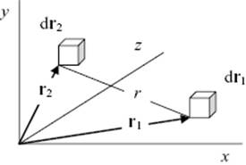
where ρ = N/V is the number density. The doublet distribution function with h = 2 describes the probability to find one molecule in dr₁ at position r₁ and another in dr₂ at position r₂ (Figure 6.4). We have now

(6.8)

Figure 6.4 The location of infinitesimal volume element dr₁ located at r₁ and the volume element dr₂ located at r₂ with their distance r.

If we assume that the potential energy can be described as the sum of two-particle potentials which are spherically symmetrical, we have for two particles at large distance ρ⁽²⁾(r₁,r₂) ≅ ρ⁽¹⁾(r₁)ρ⁽¹⁾(r₂) = ρ². For more close-by distances, we need the original expression ρ⁽²⁾(r₁,r₂), which we can write as ρ⁽²⁾(r₁,r₂) = ρ²g⁽²⁾(r₁,r₂) with g⁽²⁾(r₁,r₂) the (pair) correlation function.

For a further microscopic interpretation we note that for any microscopic property X = X_N(r) = X_N(r₁,..,r_N) depending on N (ordered) coordinates the corresponding expression for the canonical average ⟨X_N⟩ reads, using Eqs (5.39) and (6.4),

(6.9)

Suppose now that X depends on only M of the N coordinates. The number of permutations for M out of N is N!/(N − M)!M!. So, if we denote the microscopic property with the coordinates ordered from 1 to M by x_M(r₁,..,r_M) and the property with any M out of N by X_M(r₁,..,r_M), we have X_M = [N!/(N − M)!M!] x_M. From Eq. (6.5) we also know that ∫..∫ρ^(N)dr_M+1..drN = (N − M)!ρ^(M). So we obtain

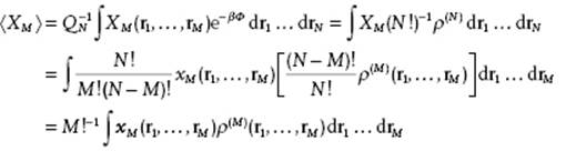
So, if X₁ = Σ_i x₁(r_i) or X₂ = Σ_ix2(r_i,r_j), we have

(6.10)

We now define the density operator D(r_i,r_i′) = Σ_i d₁(r_i) ≡ Σ_i δ(r_i − r_i′) to describe the probability that particle i is at position r_i′ and the correlation operator C(r_i,r_i′,r_j,r_j′) = ½Σ_i,j c₂(r_i,r_j) ≡ ½Σ_i,j δ(r_i − r_i′)δ(r_j − r_j′) to describe the probability that particle i is at position r_i′ while particle j is at position r_j′. Here, δ(x) is the Dirac delta function (see Appendix 2). The canonical average ⟨D⟩ = N⟨d₁(r₁)⟩ becomes ρ⁽¹⁾(r₁) according to

(6.11)

while the average ⟨C⟩ = ½N(N − 1)⟨c₂(r₁,r₂)⟩ relates to ρ⁽²⁾(r₁,r₂) according to

(6.12)

Writing ρ⁽²⁾(r₁,r₂) = ρ²g⁽²⁾(r₁,r₂), we invert to obtain

(6.13)

If there is no correlation ⟨c₂(r₁,r₂)⟩ reduces to V⁻² so that g⁽²⁾(r₁,r₂) = (1 − N⁻¹). Hence, normalization yields ∫ g⁽²⁾(r₁,r₂) dr₁dr₂ = (1 − N⁻¹) ≅ 1 for large N.

If we are not interested in the angular information contained in the set (r₁,r₂), but only in the distances, we can write ρ⁽²⁾(r₁,r₂) = ρ²g⁽²⁾(r₁,r₂) = ρ²g(r) with g(r) ≡ g⁽²⁾(r) and r = |r₁ − r₂|. From this expression we can calculate the total number of atoms N(r) in a spherical volume of radius r by integrating over both coordinates. Changing the coordinate system from (r₁,r₂) to (r₁ + r₂,r₁ − r₂) ≡ (R,r), integration over R yields the volume. The other integration over r = |r| (in a polar coordinate system) remains and we obtain after some manipulation

(6.14)

From normalization we also conclude that ∫g(r) dr = (1 − N⁻¹) ≅ 1. The integrand 4πr²g(r) is often addressed as the radial distribution function (RDF). The pair correlation function g(r) is experimentally accessible, as elaborated briefly in Section 6.3.

In the same way as for the doublet distribution function, the triplet distribution function with h = 3 can be reduced, using r_ij = |r_i − r_j|, to

(6.15)

Unfortunately, this function is not directly experimentally accessible. In general we have ρ^(h)(r₁, … ,r_h) = ρ^hg^(h)(r₁, … ,r_h).

To illustrate these ideas, let us apply them to the perfect gas for which Φ = 0 and consequently exp(−βΦ) = 1 and Q_N = V^N. Hence, for the pair distribution function

(6.16)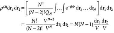

This result matches the basic probability considerations for N particles distributed randomly over a volume V because for N >> 1, Eq. (6.16) reduces to

(6.17)

This shows once more that g(r) is normalized to 1 − N⁻¹ ≅ 1 for large N.

In summarizing, if a complete set of distribution functions could be given, the description of structure would be complete, and in that case we would have a situation comparable to that of solids. However, such a set is unavailable and we must be content with just a few of them. The pair distribution function ρ⁽²⁾(r) = ρ²g(r) with number density ρ = N/V, or equivalently, the pair correlation function g(r), is the most important of these as it essentially describes the probability of finding two molecules at distance r. For independent molecules g(r) = 1 and thus ρ⁽²⁾(r) = ρ², but for correlated molecules, if it is given that the reference molecule is at the origin (with “probability” ρ), the probability of finding a molecule at distance r from the origin is given by ρg(r). Alternatively, ρg(r) describes the local density around the reference molecule.

6.2.2 Two Asides

Before discussing some experimental and simulational results on the structure of liquids, two asides should first be briefly dealt with.

The first aside is that the distribution function approach provides another means of obtaining the basic result of statistical thermodynamics, namely the Boltzmann distribution. When molecules are close together, their potential energy becomes large and positive; similarly, if the momenta are large, the (always positive) kinetic energy is also large. Hence we may suspect that a relation exists between the total energy of N molecules and the probability of a configuration as described by n^(N). So, we write . The form of can be obtained by considering the distribution function for two containers, one with N molecules and one with M molecules, which are to be combined. With distri­bution functions being probabilities, the joint distribution function reads not only but also , so that we have . This relationship can only be satisfied by , where β is a positive constant and the negative sign is required because the probabilities should remain finite for arbitrarily large values for E. Normalization leads to , while β can be obtained by applying these results to the simplest system possible, that is, an ideal gas (see Sections 5.2 and 5.3). This leads to β = 1/kT. We thus obtain

(6.18)

If we are only interested in structure but not in dynamics, and the energy expression reads , we have seen in Section 5.2 that the integrals factorize and the momenta contributions cancel from the numerator and denominator. We then have

(6.19)

The second aside deals with systems in which the number of molecules is conserved as, has been the case so far. In this situation the total number of degrees of freedom (DoF) is also conserved. Bearing this in mind, we should examine the change of a distribution function with time. The conservation of the number of DoF implies conservation of the number of phase points, that is, dn^(N)/dt = 0, resulting in

(6.20)

(6.21)

wherein the last step use has been made of and Hamilton's equations (see Section 2.2). Equation (6.21), representing Liouville's theorem (see Section 5.1), states that the distribution functions are only implicitly dependent on time.