Liquid-State Physical Chemistry: Fundamentals, Modeling, and Applications (2013)

6.4. The Structure of Liquids

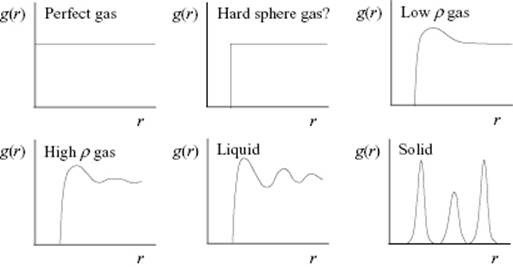
We now discuss some structural, experimental and also simulation considerations for simple and normal liquids in terms of the correlation function. While the basics of the experimental determination of g(r) is treated in Section 6.3, we refer for simulations to Chapter 9. We first compare qualitatively the behavior of g(r) for gases, liquids, and solids (Figure 6.5). For the perfect gas the density is everywhere the same, and hence no correlation is present. For a hard-sphere gas one might expect a cut-off at the hard-sphere value with no correlation for larger values of r (whether this is true or not, we will come to this point later). In a low-density real gas there is some attraction, and hence a small peak is expected at about twice the molecular radius, whereas for a high-density gas some further structure is anticipated. For a liquid, one expects even more structure as the density is comparable to that of a solid. The first peak corresponds to the first shell of atoms around the reference atom, usually indicated as the first coordination shell, while the second peak represents the second coordination shell. Finally, in the case of the solid, where atoms remain largely at their equilibrium positions, one expects clear peaks due to the largely static coordination shells.

Figure 6.5 Schematic of the pair correlation function g(r) for gases, liquids, and solids.

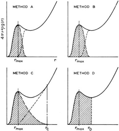
By using Eq. (6.14), it is possible to calculate the number of molecules around a reference molecule, the so-called coordination number (CN). For experimentally determined distribution functions, as only the probability is known as a function of distance, determination of the coordination number is ambiguous and several methods can be applied to obtain it. Four methods, as evaluated by Pings [5], are shown in Figure 6.6. Pings concluded that determination of the CN is somewhat arbitrary, and results obtained with different methods are difficult to compare. In practice, method D in Figure 6.6 is normally used. For the first and second coordination shells, we obtain

(6.30)

where M₁ and M₂ denote the first and second minima in the correlation function. A rough estimate for N⁽¹⁾ for dense liquids can be obtained as follows. For a dense liquid, we have approximately ρσ³ ≅ 0.64/0.74 and estimate that M₁ ≅ 2^1/2σ. Then, by using g(r) = 0 for r < σ and, say, g(r) = 1.5 for σ < r < 2^1/2σ, we obtain

(6.31)

confirming once more the relatively large CNs for liquids.

Figure 6.6 Methods of estimating the coordination number from the radial distribution function (RDF). Method A considers that the first peak in the RDF results from a symmetric rg(r), while method B considers r²g(r) as symmetric. Method C uses the extension from the first maximum to the distance where the RDF is continuously increasing. Method D simply uses the first minimum in the RDF.

So, close to the triple point, the density of a liquid resembles that of a random close packing of spheres with η ≅ 0.64 and N⁽¹⁾ ≅ 10, compared with η = 0.74 and N⁽¹⁾ = 12 for the FCC lattice, and implying an expansion of ∼15% upon melting. It appears that, near the critical point, the intermolecular spacing for a wide range of liquids is given by l = (V_cri/N)^1/3 = (1.50 ± 0.16)σ. This implies a linear expansion from σ near the triple point to 1.5σ near the critical point, or a volume expansion by a factor of 3.4. This amount of expansion cannot occur by a rearrangement of the local coordination, but rather requires the introduction of holes of molecular size. This leads to a lower CN, although the nearest-neighbor distance is changed only slightly.

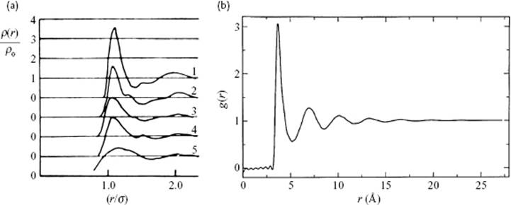
Some early experimental data, as well as more sophisticated measurements for Ar at various temperatures, are shown in Figure 6.7. This figure shows the structure anticipated with a clear first coordination shell. It is also possible to recognize a second coordination shell and, for lower temperature, also a third shell. Thereafter, the structure becomes “fuzzy,” indicating the essentially random nature of liquids. These figures also show the rapid fading out of structure with increasing temperature. Finally, when comparing Figure 6.7a with Figure 6.7b, the considerable improvement in experimental results over the years becomes very clear.

Figure 6.7 (a) Correlation of Ar as measured using X-ray diffraction [9]. Labels: 1 = 84.4 K (∼ triple point); 2 = 91.8 K; 3 = 126.7 K; 4 = 144.1 K; 5 = 149.3 K (∼ critical point). The size of Ar is σ = 3.42 Å; (b) Correlation function as determined using neutron ray diffraction (NRD) at 85 K [10].

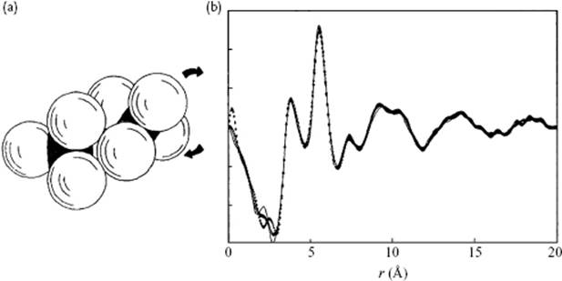
In Figure 6.8 the correlation function for a molecular liquid, namely N₂, is presented. In Figure 6.8a, the experimental correlation function, as obtained using NRD experiments, is shown, whereas in Figure 6.8b the intermolecular correlation function (this means that the intramolecular N–N distance is not shown) for this liquid is given, as obtained from a molecular dynamics (MD) simulation (see Chapter 9) of 256 rigid molecules interacting via a Lennard-Jones potential. Again, the structure fades away with increasing temperature. The CN obtained was about 12 throughout the temperature range under consideration. The structure used and the main configurations for the N₂ dimers analyzed are shown in Figure 6.9. It appeared from these calculations that the R- and T-configurations occurred each for 47–48%, while the S-configuration occurred for only about 3%, independent of the temperature (in the range of 70 to 120 K) and the assumed ratio of the moments of inertia I_z (along the molecular axis) versus I_x and I_y (perpendicular to the molecular axis). It is clear that the interpretation of the pair correlation function of molecular liquids requires an insight into their chemical structures before conclusions can be drawn regarding the liquid structure. Results similar to those with N₂ have been obtained for several other systems; an example can be seen in Figure 6.10, which shows liquid phosphorus containing P₄ molecules.

Figure 6.8 (a) The intermolecular correlation function of N₂ as obtained from rigid molecule molecular dynamics simulations at 80 K (solid line, ρ = 0.796 g cm⁻³), 100 K (dotted line, ρ = 0.689 g cm⁻³), and 120 K (dashed line, ρ = 0.525 g cm⁻³). The parameters used were: nuclear distance L = 1.098 Å, σ = 3.341 Å, and ε = 0.6064 × 10⁻¹⁴ erg [11]; (b) The (total) correlation function of N₂ as obtained from NRD experiments, showing both the intra- and intermolecular distances [12].

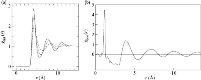
Figure 6.9 (a) The assumed structure with nuclear distance L and Lennard-Jones diameter σ; (b) Main configurations R, S, and T, as used for a molecular dynamics simulation of N₂.

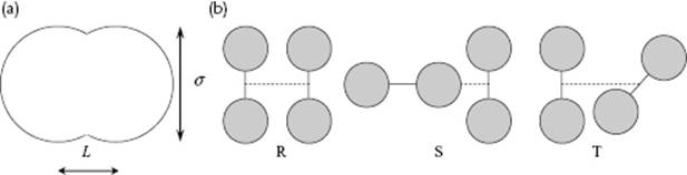
Figure 6.10 (a) The interlocking of XY₄ molecules; (b) The (total) experimental correlation function of P₄ as obtained from NRD experiments, showing as the first peak the P–P distance of the atoms in contact and as the second peak the P–P distance as arising from the interlocked configuration [12].

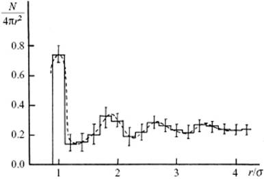
Before embarking on the related energetics, it should be mentioned that a number of attempts have been made in the past to simulate the (static) structure of a monoatomic liquid using analogous models, providing a static – though qualitatively correct – picture of the structure of liquids. In particular, packings of steel balls (as used in ball bearings) have been used. From the well-defined random closed-packed assemblies of these balls, Bernal [6] (actually his assistant) was able to determine the pair distribution function by counting their numbers with increasing distance from a reference ball, and averaging over several reference balls. The thus-obtained pair correlation function closely resembled the experimentally determined correlation functions for mono-atomic liquids, such as argon and several metals. The somewhat more elaborate results as obtained by Scott, are shown in Figure 6.11 [7]. The CN was also determined using an interval from 1.0σ to 1.2σ, where σ is the sphere diameter, which led to values of about 9.3 ± 0.8. In this case, determination of the CN was relatively straightforward (though tedious!), and subsequent computer simulations [3] essentially confirmed these findings. It should be borne in mind, however, that analogous models can provide a static picture of liquids, while the nature of fluids is essentially dynamic.

Figure 6.11 The pair correlation of the hard-sphere fluid as determined experimentally by Scott [7] from an assembly of close-packed steel balls.

Problem 6.2

Verify Eqs (6.4), (6.5), and (6.14).

Problem 6.3

Calculate the pair correlation function for a solid with the simple cubic (SC) structure. Do the same for a solid with FCC structure, a solid with the HCP structure, and a solid with the BCC structure.

Problem 6.4

Calculate the CNs from the pair correlation function as given by Scott for the first and second coordination shell using method D in Figure 6.6.

Problem 6.5

Show that is the only solution of .

Problem 6.6

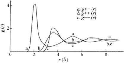
The pair distribution function [8] for molten LiCl, as calculated via MD simulations, is shown in the accompanying figure. The (Pauling) ionic radii for the Li⁺ and Cl⁻ ions are 0.61 Å and 1.81 Å, respectively. Crystalline LiCl has the NaCl structure with lattice constant 5.14 Å.

a) What is the “nearest-neighbor” and “next-nearest-neighbor” distance’ between the Li⁺ and Cl⁻ ions (the Li–Cl pair)?

b) What are the “nearest-neighbor” distances for the pairs Li–Li and Cl–Cl?

c) At first sight, one could expect that the Li–Li distance would be about 1.2 Å, and the Cl–Cl distance about 3.6 Å. However, the pair distribution function for the molten state indicates that these “nearest-neighbor” distances in the liquid are about the same. Discuss why this is so.