Liquid-State Physical Chemistry: Fundamentals, Modeling, and Applications (2013)

7.2. Integral Equations

In the previous section, as well as in Chapter 6, we have seen that the pair correlation function g(r) is the essential unknown. So, let us see whether we can obtain a theoretical expression for the correlation function g(r). There are several approaches to achieve this goal. We deal first with the Yvon–Born–Green equation, and continue with the Kirkwood equation. After introducing some new concepts leading to the Ornstein–Zernike equation, we introduce briefly the hypernetted chain, Percus–Yevick, and Mean Spherical Approximation approaches. Those readers not interested in the details of the various approaches should consider them simply as labels for particular approximate solutions in the paragraph comparing results, and in Section 7.3.

7.2.1 The Yvon–Born–Green Equation

The eldest – and, in principle, the most clear approach – runs as follows. We start with the pair distribution function (see Chapter 6) with, as before, β = 1/kT

(7.4)

We assume again that the potential energy is pairwise additive, Φ = ½Σ_ijϕ_ij, and differentiate with respect to r₁. Since the integration is over r₃ to r_N and differentiation is with respect to r₁, differentiation and integration can be exchanged to yield

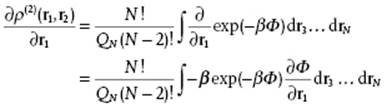
Because we assume that Φ = ½Σ_ijϕ_ij = ϕ₁₂ + … + ϕ_1N + ϕ₂₃ + … + ϕ_N−1,N we obtain so that

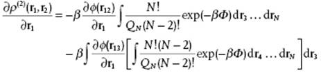
In the first integral we recognize ρ⁽²⁾ and in the one in square brackets ρ⁽³⁾ and, if we divide by ρ² and use ρ ⁽²⁾ = ρ²g⁽²⁾ and ρ ⁽³⁾ = ρ³g⁽³⁾, the overall result is

(7.5)

This is an infinitely nested set of coupled equations that is usually denoted as the Yvon–Born–Green (YBG) hierarchy [2], and which can be solved formally by iteration. However, for a concrete solution a “closure” is required, and to that purpose we employ the potential of mean force W⁽³⁾(r₁, … , r₃), as discussed in Section 6.3. Suppose that we assume – not completely unrealistically – that this potential of mean force for triplets is to a first approximation pair-wise additive, that is, W⁽³⁾(r₁,r₂,r₃) ≅ W⁽²⁾(r₁,r₂) + W⁽²⁾(r₂,r₃) + W⁽²⁾(r₃,r₁). This results in

(7.6)

Using this superposition approximation, as originally proposed by Kirkwood and Boggs [3] as a closure relation for the YBG hierarchy, leads to an integral equation which can be solved numerically. The resulting YBG equationreads

(7.7)

showing again that: (i) the potential of mean force W = −kTlng is composed of the direct interaction ϕ(r₁₂) and the weighted interaction on particle 1 exerted by all particles 3 at arbitrary positions; and (ii) W = −kTlng reduces to ϕ for ρ → 0.

Of course, this approach can be used for ρ⁽ⁿ⁾ with n ≠ 2, but let us here generalize slightly the meaning of Φ. So far, Φ only included the pair potential contributions, that is, Φ = ½Σ_ijϕ_ij, but in several problems there is also an external potential X acting on each molecule individually, that is, X = Σ_i χ_i. Repeating the proce­dure outlined above, but now for n = 1 and including Φ and X, we obtain (using ρ ≡ ρ⁽¹⁾)

(7.8)

If Φ may be neglected, for example, as for a dilute gas, we are left with X result­ing in

(7.9)

Taking for χ the potential due to gravity, χ = mgh, we obtain the well-known barometric formula with ρ(0) the density at h = 0.

7.2.2 The Kirkwood Equation*

Another relatively old approach uses thermodynamic integration in combination with the pairwise additivity assumption Φ = ½Σ_ijϕ_ij. We start again with the distribution function (with, as before, β = 1/kT), but this function is now dependent on the coupling parameter ξ, that is,

(7.10)

In this case we differentiate with respect to ξ to get

(7.11)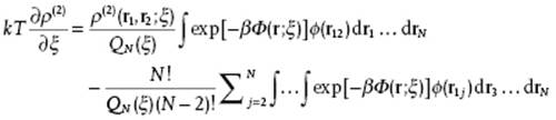

The first term can be written as

(7.12)

while the second term involves two separate cases. For j = 2, the factor ϕ(r_1j) can be taken outside the integral resulting in

(7.13)

For j = 3, … , N, the result is

(7.14)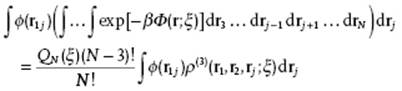

Taking these results together and dividing by ρ⁽²⁾(r₁,r₂) yields

(7.15)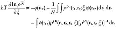

The next step is to integrate the previous equation from 0 to ξ meanwhile using

(7.16)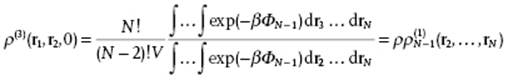

where denotes the distribution function for system containing N − 1 molecules.¹⁾ Integration thus gives after some manipulation

(7.17)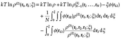

Introducing the correlation functions g⁽²⁾ and g⁽³⁾ the final result becomes

(7.18)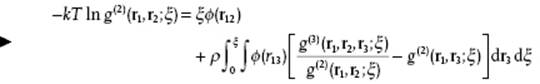

This expression gives g⁽²⁾ in terms of g⁽³⁾ and provides another example of a hierarchy of coupled equations, the so-called Kirkwood (K) hierarchy [4]. Again, using the superposition approximation results in the Kirkwood equation

(7.19)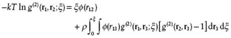

Also this integral equation has to be solved numerically and shows again that for ρ → 0, W = −kT ln g → ϕ. It can be shown that the YBG and K hierarchies are equivalent [5], but that the approximate solutions to the YBG and K equations are not.

7.2.3 The Ornstein–Zernike Equation*

For the following, it is convenient to introduce some auxiliary functions. Since we consider isotropic systems we use r_ij = |r_j − r_i|, or even r if confusion is impossible. In this notation the expressions for the pair correlation function g(r₁,r₂) and the often-used Mayer function f(r₁,r₂) using e ≡ exp[−βϕ(r₁,r₂)] become

with Φ and ϕ the total potential energy and two-particle potential energy, respectively.

To introduce the auxiliary concepts, we recall that ρg(r₁₂) = ρg(r₁,r₂) describes the probability of finding a particle at distance r₁₂ = |r₂ − r₁| from the origin, given that another particle is located at the origin. No correlation would intuitively imply g → 0 for r₁₂ → ∞, but for r₁₂ → ∞ we actually have g → 1. Therefore, we define the so-called total correlation function by h(r₁₂) ≡ g(r₁₂) − 1, for which obviously holds: r₁₂ → ∞, h → 0. The total correlation between particle 1 and particle 2 is supposed to be composed of two contributions:

· the direct correlation between particles 1 and 2, represented by the direct correlation function c(r₁₂); and

· the indirect correlation of particle 1 and particle 2 via the influence of particle 1 on particle 3 and the influence of particle 3 on particle 2 summed over all such third particles (with density ρ). This results in the convolution ρ∫c(r₁₃)h(r₃₂) dr₃.

The total correlation is thus given by

(7.20)

This so-called Ornstein–Zernike (OZ) equation, originally used by these authors in 1914 to explain light scattering in liquids near the critical temperature, is in fact one way of defining the direct correlation function c(r₁₂). Although the physical interpretation of c(r₁₂) is not as clear as that for g(r), it does have a simpler structure, and in particular it has a much shorter range. A formal solution can be obtained by iteration yielding

(7.21)

This solution can be interpreted as a sum of “chains” of direct correlation functions between r₁ and r₂. Since the OZ equation is a convolution, a practical solution for h(r₁₂) can be obtained from its Fourier transform (see Appendix B). Using

(7.22)

we obtain

(7.23)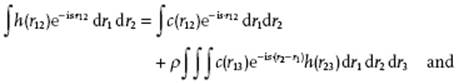

(7.24)

The direct correlation function is connected to the compressibility equation, Eq. (6.33). This can be seen if we rewrite the compressibility equation

(7.25)

(7.26)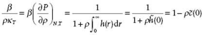

where Eq. (7.22) with s = 0 is used. For both c(r) and g(r) = h(r) + 1, expansions in ρ can be formulated for which we refer to the literature (e.g., Ref. [6]).

So far, we have introduced several functions, which will be used again in the sequel, and for convenience we summarize them here. As before, ϕ denotes the pair potential, β = 1/kT, and ρ is the number density.

(7.27)

(7.28)

(7.29)

(7.30)

(7.31)

(7.32)

(7.33)

(7.34)

In order to be concise, we omit in the following two paragraphs largely in the arguments for each of these functions, except when it is required to be precise.

7.2.4 The Percus–Yevick Equation*

The integral equations to be discussed can be derived in various ways, for example, by systematic expansion using the so-called (graphical) cluster expansion or by functional differentiation [7, 8]. Here, we use another entrance as described by McQuarrie [6], using the OZ equation. In order to solve the OZ equation for either c(r) or h(r), we need another relation, a “closure”, between c(r) and h(r).

To that purpose we consider the direct correlation function c(r) to be the difference between the correlation function g(r) = exp[−βW(r)] and an indirect correlation function g_ind(r). Using the potential of mean force W(r), we approximate g_ind(r) by g_ind(r) ≅ exp[−β(W − ϕ)]; that is, we assume – not unreasonably – that the potential of mean force W minus the pair potential ϕ provides a good estimate for g_ind. Hence, we use the approximation

(7.35)

where the background correlation function y = g/e is used.

The Percus–Yevick (PY) approximation, named after its originators, results from this approximate closure relation for the OZ equation. For c and h we then have the equivalent forms

(7.36)

Inserting h = c + y − 1 into the OZ equation, we obtain

(7.37)

Since f is known, this integral equation in y, known as the PY equation, can be solved numerically for y and, once y is obtained, this leads directly to g = ye.

7.2.5 The Hyper-Netted Chain Equation*

The Hyper-Netted Chain (HNC) equation is obtained by expanding y = exp[−β(W – ϕ)] to first order, so that y = 1 − β(W − ϕ). Hence, from c = g − y we have the various equivalent forms

Inserting c = h − ln y into the OZ equation results in one form of the HNC equation

(7.38)

(7.39)

This integral equation in g, since e and ϕ are known, can be solved numerically.

The HNC approximation received its name from the types of diagram that are included in the graphical cluster expansion analysis (these are not discussed here). Although from this presentation it appears that the HNC equation is an approximation to the PY equation, the more sophisticated cluster expansion analysis shows that this is not true. While the HNC approximation neglects certain terms in the expansion because of their complexity, the PY approximation neglects even more terms. However, the original, physical derivation of the PY equation is in terms of “collective coordinates,” resembling the harmonic analysis of a crystalline solid [9]. While the HNC equation is thus a pure mathematical approximation, the PY equation has some physical basis.

7.2.6 The Mean Spherical Approximation*

The mean spherical approximation (MSA) consists of the core condition g(r) = 0 for r < σ and the approximation c(r) = −βϕ(r) for r > σ, together with the OZ equation. For hard-spheres with ϕ(r) = ∞ for r < σ, where σ is the hard core diameter, this approach is identical to the PY approach and an analytical solution is possible (see Section 7.3). However, the importance of the MSA approximation is contained in the fact that it can be solved analytically for other cases. In particular, if ϕ(r) represents the ion–ion or dipole–dipole interaction, a solution can be found using Laplace methods. These solutions are used in the description of models for ionic solutions and polar fluids.

7.2.7 Comparison

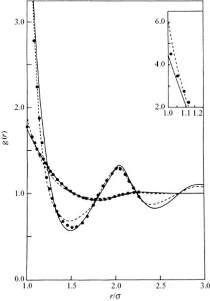
In this paragraph we illustrate the results of some integral equation calculations. As before, we use the number density given by ρ = N/V and the packing fraction reading η = ρb/4 = πσ³ρ/6 with b = 2πσ³/3. The results of integral equation calculations for the hard-sphere fluid at low (η = 0.21) and high density (η = 0.47) are shown in Figure 7.1, and compared with Monte Carlo (MC) simulation results. From the figure it is clear that both the PY and HNC approximations result in a similar pair correlations function as the MC simulation. For low density, g(r) falls monotonically until it reaches about 1.8σ, shows a small second maximum, and thereafter g(r) ≅ 1. The large first peak represents the nearest-neighbor distance, and for this density it is clear that the structure becomes rapidly random. For high density there is more structure in g(r) with clear second and third neighbor distances. Although the correlation functions using the PY and HNC approximations are qualitatively quite satisfactory, there are two defects when compared to the MC simulation. First, the value at contact is too low for the PY solution and too high for the HNC solution. Second, the oscillations are slightly out of phase for both the PY and HNC solutions.

Figure 7.1 The pair correlation function for a hard-sphere fluid. Results shown are: - - -, HNC; −−−, PY; ••••, Monte Carlo. The curves with the smaller intercept represent a state with η = 0.21, while the other curves represents a state with η = 0.47 (intercept shown in inset).

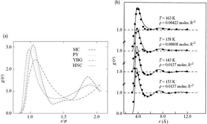
The results for a Lennard-Jones fluid [10] at η = 0.58 and T_red = kT/ε = 2.74, using the PY, YBG, and HNC approximations, are shown in Figure 7.2, and compared with MC results. Similar to the hard-sphere fluid, the overall behavior of the calculated results mimics the MC results reasonably well, although clear differences can be noticed. The YBG result mimics the MC results poorly for the second coordination shell, and all peaks in the calculated results are displaced with respect to the MC results. Figure 7.2 also shows the comparison of PY results with experimental data for Ar. The qualitative features are well reproduced, although some differences can be noticed particularly at low densities. It is probably also clear that the influence of density is more pronounced than that of temperature, which is to be expected because the structure is largely determined by the repulsive forces.

Figure 7.2 (a) The correlation function g(r) for a Lennard-Jones fluid at η = 0.58 and T_red = kT/ε = 2.74, calculated using various methods; (b) The correlation function g(r) for Ar using the PY approximation [29] compared to experimental data [30].

Whilst various authors do not always agree on the merits of the PY and HNC approximations, it is clear that both are superior to the YBG approximation. For example, Watts and McGee [11] stated that the PY approximation “… can be derived from physical arguments and is superior to the HNC approximation for many problems”. Oppositely, Fawcett [12] remarked that the “… HNC equation provides a better description of most systems than the PY equation”. Nowadays, the PY approximation is often considered to be the best approximation to the solution of the integral equation describing simple liquids with strong repulsions and short-range interactions. For systems with long-range interactions, however, the HNC equation appears superior.

Problem 7.2*

Derive Eqs (7.24), (7.37), (7.38) and (7.39).