Liquid-State Physical Chemistry: Fundamentals, Modeling, and Applications (2013)

8.2. Cell Models

Kirkwood contemplated how to rationalize cell models (a somewhat complex process schematically discussed in Justification 8.1), but long before that Lennard-Jones and others used the cell model to obtain both analytical and numerical results.

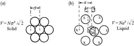
Hence, let us use a cell model with a lattice-like structure in which we introduce some free volume. As the density of a liquid deviates not too much from the solid, we use for the lattice a dense close-packed lattice such as the FCC lattice structure (Figure 8.2) with hard-sphere atoms. In a FCC lattice, the volume per molecule is v₀ = V₀/N = σ³/γ, where γ = 2^1/2 and σ is the molecular diameter. For other lattices we will have different γ-values. Expanding this lattice slightly, we have a³/γ = v = V/N. The configuration integral for the wanderer, labeled as molecule 1, represents the volume available to the wanderer, weighted with a Boltzmann factor, that is, the free volume, reads

(8.1)

where the integration is in principle overall space, although as the wanderer cannot leave the cell, it may be taken over the cell. If the wanderer is inside the cell, the potential energy ϕ(r₁) = 0 because the atoms are considered as hard-spheres and therefore we have exp(−ϕ/kT) = 1. Since the wanderer cannot be outside the cell, for |r₁| > a the potential energy ϕ (|r| > a) = ∞, leading to exp(−ϕ/kT) = 0. If we assume that we may replace the cell by a sphere of radius (a−σ), we obtain for Q(1)

is the expression for the free volume per molecule for this particular model. More complex potentials will result in different expressions for the free volume. Given this result, the configurational Helmholtz energy for the wanderer becomes

(8.2)

or since any molecule can be the wanderer we obtain the expression for the liquid by taking N times the expression for F_con(1)

(8.3)

Figure 8.2 A two-dimensional representation of the FCC lattice for the solid state (a) and the liquid state (b) in which the distance between the atoms has been increased from σ to a so that the “smeared” diameter of the free volume, indicated by the hatched hexagon, becomes a − σ.

Because P = −∂F/∂V and in F = F_kin + F_con ≡ −kT lnΛ^−3N − kT ln[Q(1)^N], only F_con depends on V, and we have

(8.4)

The limiting behavior of this simple equation is not too bad. If V → V₀, P → ∞ (which means that at high pressure the behavior is approaching the solid state). If V becomes large, P → NkT/V, as it should do. However, in the neighborhood of the triple point, PV/NkT << 1 but the expression on the right-hand side appears to be >> 1 because V₀/V is typically 0.8. The origin of this failure is simple: the model contains no attractive interaction. The simplest way to introduce attraction, based on empirical insight [5], is to use for the average potential ϕ(0) the expression

(8.5)

with a(T) ≥ 0 a parameter that is dependent on temperature only, leading to

(8.6)

This results in

(8.7)

and via P = −∂F/∂V to

(8.8)

This expression, often denoted as the Eyring EoS, is a significant improvement of the cell model, resembling the van der Waals equation, Eq. (3.5), (P + a/V²)(V − b) = RT, where a and b are parameters, and gives a useful semi-empirical description of liquids.

A more sophisticated cell model was proposed by Lennard-Jones and Devonshire [6], here labeled as the LJD theory. In this model, again the FCC lattice is used but now in conjunction with the Lennard-Jones potential ϕ_LJ(r) with equilibrium distance r₀ = 2^1/6σ and depth ε. In the original LJD model the interaction of the wanderer with its z = 12 nearest-neighbors is calculated by supposing again that the neighbors are distributed with equal probability over a sphere with radius a = (γV/N)^1/3 ≡ (γ/ρ)^1/3 using a cell radius a₁ ≥ 0.5a. For this spherical cell the potential ϕ is then a function of the distance r from the center of the cell only. At the center we have the potential

(8.9)

while for a position off-center an extra contribution Ψ(r) has to be added, that is, ϕ(r) = ϕ(0) + Ψ(r). The authors showed that, using ,

(8.10)

(8.11)

(8.12)

(8.13)

The partition function Q = Q(1)^N becomes (using β = 1/kT)

(8.14)

The choice of a₁ depends on the “smearing” assumptions. It appears that Ψ(r) becomes large and positive for r → 0.5a. Lennard-Jones and Devonshire therefore took a₁ = 0.5a. Because the introduction of the more realistic LJ potential complicates the matter²⁾, the necessary integrations must be performed numerically.

The model predicts sinuous curves for the pressure below and monotonic curves above a certain temperature. Identifying this temperature as the critical temperature, the model predicts (using the LJ potential) for the critical constants

(8.15)

to be compared with the best experimental corresponding states estimates

(8.16)

We see that the value of T_cri is about right, the value for V_cri too small by a factor of about 2, and P_cri too large by a factor of about 4.

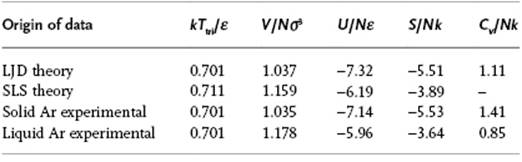
It is not very realistic to expect that the wanderer will be permanently confined to the cell at or near the critical temperature. One might expect that at low temperature, perhaps at or near the triple point, this is assumption is more realistic and agreement with experiment is better. For Ar, the triple point temperature is 0.701ε/k, and at this temperature the pressure is so low that the molar volume may be obtained by setting P = 0 in the equation of state (EoS). Table 8.1 provides some data for Ar at the triple point. It is concluded that, on the whole, the values of the properties calculated with LJD theory are much closer to the experimental values for solids than for liquids, as might be expected.

Table 8.1 Data for Ar at the triple point T_tri. Experimental data taken from Ref. [4].

Later authors [8] included non-nearest-neighbor effects for ϕ(0) and v_f via a lattice sum³⁾ calculation, but this did not lead to any significant improvement. These authors also chose a₁ according to , that is, the volume of the cell equals the volume per molecule, or a₁ = 0.5527a. The precise choice appears to be noncritical. On the whole, this conceptual improvement does not bring about any significant improvement in agreement with experiment. Also, the “smearing” approximation for v_f for hard-spheres appeared to have a limited influence [9]. Allowing the double occupancy of cells leads to somewhat improved results [10]. The thermodynamic properties as calculated by the LJD method appear to be insensitive to the precise potential used [11]. Finally, we note that cell model calculations have been made using a random close-packed structure and employing the LJ potential [12]. The results for energy compare favorably with MC and MD results, although the results for pressure appear to be rather sensitive to the correlation function used. Extending this model by using a nonzero probability for being off-center for all molecules removes the basic inconsistency mentioned in Section 8.1, and leads to somewhat improved results [13].

An important deficit of this type of models is the communal entropy problem, which is due to the assumption that the wanderer cannot leave the cell. To illustrate this problem, consider a gas. The correct partition function for the ideal N-atom gas is given by, using Λ = (h²/2πmkT)^1/2,

(8.17)

so that the Helmholtz energy reads

(8.18)

For the cell model the partition function for the wanderer is given by

(8.19)

so that the Helmholtz energy for N atoms in the cell model is

(8.20)

The difference between these two expressions constitutes the communal Helmholtz energy which we calculate from

(8.21)

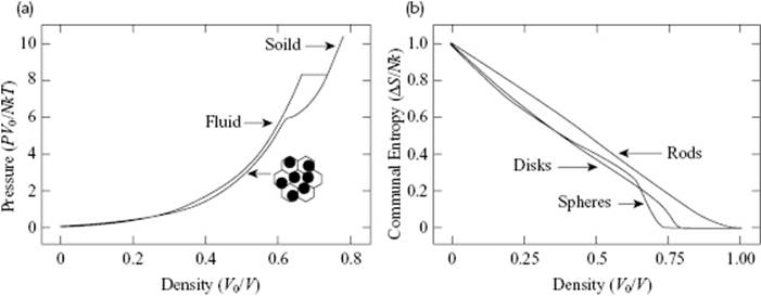
Hence, for one mole the cell model estimates the molar entropy too low by Δ_comS = R. The basic reason for this is the limited volume that an atom can probe in the cell model (the cell volume) as compared to the volume probed in reality (the complete volume). Obviously, the same argument applies also to liquids, because we know that in liquids the atoms can move to any position, albeit somewhat restrictedly. For solids, where the atoms essentially remain at their positions, the approach would be correct and the cell model is thus describing a solid-like situation rather than a liquid-like situation. Eyring [14] made the rather arbitrary assumption that the communal entropy would be completely released during melting, which would lead to an (extra) communal entropy factor e^N in the partition function Z_N. In this way, the limiting behavior for gases becomes correct. The communal entropy Δ_comS issue was resolved by Hoover and Ree [15] by using Monte Carlo simulations (see Chapter 9) for hard-spheres. They essentially calculated Δ_comS by subtracting from the entropy for the unconstrained, normal hard-sphere fluid that of a constrained fluid. In the latter model each sphere can move only within its own cell, in similar fashion to the cell model and consistent with the definition of communal entropy as given by Kirkwood (see Justification 8.1). Data for varying sizes were extrapolated to those for an infinite system, and from these calculations it appeared that the hard-sphere (disordered) fluid and (ordered) solid phases are in equilibrium with densities ρ_L = (0.667 ± 0.003)ρ₀ and ρ_S = (0.736 ± 0.003)ρ₀, respectively, where ρ₀ is the close-packed density. The melting pressure and temperature are related by P_M = (8.27 ± 0.13)ρ₀kT_M (Figure 8.3). Hence the hard-sphere solid expands by about 10% upon melting. The density of the solid shows a cusp at 0.637ρ₀ where the cell walls begin to become important. At this point, the crystal becomes mechanically unstable and without the walls it would rapidly disintegrate. It also appeared that Δ_comS decreases approximately linearly from Δ_comS = 1.0Nk at ρ = 0, corresponding to the factor e^N in Q, to Δ_comS = 0.2Nk at ρ = 0.65 ρ₀ (Figure 8.3). There is no simple way to either solve or circumvent the communal entropy problem for cell models, although some other approaches (e.g., hole models) do so (Section 8.3).

Figure 8.3 The equation of state for three-dimensional (3D) hard-spheres for the fluid and solid states, where the solid and fluid isotherms are connected by a tie line at equal chemical potential at PV₀/NkT = 8.27 (a) and the communal entropy for 1D, 2D, and 3D hard-spheres (b).

Justification 8.1: Kirkwood's analysis*

Consider, like Kirkwood [16], a system of N interacting identical particles with partition function Z_N ≡ (Λ^3NN!)⁻¹Q_N. Let us divide the coordinate space into N cells Δ₁,Δ₂, … ,Δ_N, each of volume Δ, in an arbitrary manner. The configuration integral then becomes a sum of terms in which the coordinates of the molecules are confined to a particular cell. Thus, Q_N will contain N^N integrals, corresponding to the N^N ways of positioning N molecules in N cells. Hence

(8.22)

with Φ = Σ_i<jϕ_ij. Now denote by Q_N(m₁,m_2,… ,m_N) the various terms in Eq. (8.22) corresponding m₁ molecules in cell 1, m₂ molecules in cell 2, … m_N molecules in cell N. Because the molecules are identical, there are (N!/Π_i m_i!) ways of obtaining a particular set {m} = m₁,m_2,… ,m_N. Therefore, Q_N becomes

(8.23)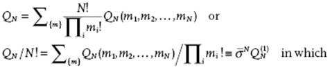

(8.24)

The summation is over all sets {m} subject to the constraint Σ_i m_i = N. At sufficiently high densities the repulsive interaction prevents multiple occupancy, so that all Q_N(m₁,m₂, … ,m_N) are zero except and . On the other hand, for highly dilated gases there is effectively no interaction between the molecules and all Q_N(m₁,m₂, … ,m_N) are equal. Hence, so that using Stirling's approximation, or . Hence, generally and its change with density represents the communal entropy. The derivative of with respect to Vcontributes to P. To make the next step we need the probability density

(8.25)

where is the configurational partition function for a system of N interacting molecules, each of which is required to remain in its particular cell. We approximate by a product of functions s(r_i), each dependent only on the coordinates of one molecule r_i with respect to the origin in the cell, that is,

(8.26)

The optimum choice for s(r_i) is obtained by minimizing F = U − TS at constant T and Δ subject to the normalization constraint of s(r_i). Here

(8.27)

where is the configuration Helmholtz energy for N interacting molecules restrained to their cells. As shown in Chapter 5, the configuration energy and entropy are given by, respectively,

(8.28)

Therefore, F⁽¹⁾ becomes (after some manipulation)

(8.29)

with Y(r) = Σ_j=2ϕ (R_1j − r) as the contribution to the potential energy due to molecule 1 at position r with respect to the origin of cell 1 with all other particles located at their respective origins, and R_1j contains the origins of all j cells with respect to the origin of cell 1. To find the optimum we need to solve

(8.30)

Using Lagrange multipliers leads (again after some manipulation) to

(8.31)

(8.32)

(8.33)

This solution provides the best approximation to in terms of s(r). The total partition function Z_N and the free volume v_f then become

(8.34)

From these expressions the thermodynamic properties can be obtained in the usual way after a choice for and Ψ(r) is made. As zeroth approximation, we assume that the molecules are located at the center of their cells and, using the Dirac delta function, we have s(r) = δ(r), leading to

(8.35)

Restricting the sums to nearest-neighbors, replacing this sum by an integral over a sphere of radius equal to the nearest-neighbor distance and taking yields the LJD model. We have Y₀ = zϕ(0) and Ψ(r) = z[ϕ(r) − ϕ(0)] and the results become

(8.36)

Although this analysis represents a significant step in theory, it is also clear that the problem lies in evaluating . An expression for may be based on the MC results of Hoover and Ree, but such an approach remains empirical.

Problem 8.1

Derive the expressions for U, S, and μ from Z for the simple cell model.

Problem 8.2: Free volume via sound velocity

The free volume in a liquid can be estimated using the speed of sound in the liquid. In a simple model we use three molecules A, B, and C in a straight line. If a sound wave travels from left to right, molecule A collides with molecule B and the signal is transferred instantaneously to the opposite side of molecule B. Thus, although molecule A travels only the distance a−d in order to strike molecule B, the sound wave effectively travels the distance a.

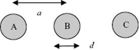
a) Estimate the ratio of the sound velocities in the gas v_G and liquid v_L.

b) Given that v_L/v_G ≅ 5, estimate the fraction of free volume in the liquid.

c) Using this model estimate the volume expansion when the solid melts. Hint: Use the free volume expression as used in the simple cell model.

Problem 8.3: Free volume via α_P and κ_T

a) Using the Helmholtz energy F for the cell model with average attraction potential ϕ and the appropriate Gibbs–Helmholtz expression, show that the internal energy is given by U/N_A = −ϕ + 3kT/2.

b) Using the Helmholtz energy F and P = −∂F/∂V, show that P = ∂ϕ/∂V + kT ∂lnv_f/dV.

c) Differentiating P with respect to T while keeping V (and N) constant and remembering that ϕ and v_f are supposed to be functions of V only, show that (∂P/∂T)_V,N = k ∂lnv_f/dV.

d) From the definition of the expansivity α_P and compressibility κ_T, show that (∂P/∂T)_V,N = α_P/κ_T.

e) Using , show that .

f) Taking the average value for normal liquids α_P ≅ 1 × 10⁻³ K⁻¹ and κ_T ≅ 1 × 10⁻⁴ bar⁻¹ together with R = N_Ak = 82 bar cm³ K mol⁻¹, show that for chloroform (V_m = 80 cm³ mol⁻¹) V_f = N_Av_f ≅ 0.44 cm³ mol⁻¹.

Problem 8.4: Free volume via Δ_vapH

It appears empirically that the vapor pressure P over a wide temperature range can be given by P = a exp(−Δ_vapH/RT), where Δ_vapH is the enthalpy of vaporization. The value of a is (nearly) constant and does not vary considerably over a range of (normal) liquids. Using the average value a ≅ 2.7 × 10⁷ atm (correct to within a factor 2), show that Δ_vapH/kT_n = ln a ≅ 10.4. Also show that for chloroform, using the same data as in Problem 8.3, V_f ≅ 1.0 cm³ mol⁻¹.

Problem 8.5: Vapor pressure

Consider the cell model with average attraction potential ϕ(T) so that the total attraction Φ_lat = Nϕ represents the energy of evaporation of the liquid. Using the partition function given by Eq. (8.6), calculate the chemical potential μ for the cell model. Show that, by equating the chemical potential for the liquid and the (perfect) gas, the calculation for the vapor pressure P_vap results in P_vap = (kT/v_f) exp[−ϕ/2kT].

Problem 8.6: Hildebrand's rule and Trouton's constant*

The result of Problem 8.5, assuming for the liquid phase and ΔU = Δ_vapH − RT = a/V, can be used to (approximately) validate Hildebrand's rule and to estimate the value of Trouton's constant (see Section 16.2).

a) Use the Eyring EoS Eq. (8.8) in combination with to obtain an explicit expression for v_f, neglect the external pressure P with respect to the internal pressure a/V² and show that the result is ζPV/RT = [Δ_vapH/RT − 1]⁻¹ exp(−Δ_vapH/RT) with ζ = (4π/3)^1/3.

b) This result appears to be a universal function of Δ_vapH/RT for many compounds. Show that this result leads to Hildebrand's rule (see Section 16.2).

c) By realizing that the factor V varies only slightly from compound to compound in comparison with the exponential factor, show that the number density ρ is a universal function of Δ_vapH/RT.

d) Show that, by approximating R/ζV by a constant and using the typical value V_m = 80 cm³ mol⁻¹ at T = 300 K, one obtains Trouton's constant Δ_vapH = RT_n = C with C ≅ 10.4, where T_n is the (normal) boiling temperature at P = 1 atm. Show that C is insensitive to the precise value of ζ.