Liquid-State Physical Chemistry: Fundamentals, Modeling, and Applications (2013)

In Chapters 7 and 8 the integral equation and physical model approaches were introduced. Now, we outline the basics of modern simulation methods that have become feasible because nowadays sufficient computer power is available. After some preliminaries, we deal first with molecular dynamics (MD) and show the results of some early studies. Because this method essentially solves Newton's equations of motion as applied to molecules, the method is capable of calculating the structure, properties and dynamics of liquids. Next, we briefly introduce the Monte Carlo (MC) method, which essentially is a statistical method capable of calculating the static structure and properties. Finally, a typical example com­bining ab-initio quantum-mechanical results with Monte Carlo simulations is discussed.

9.1. Preliminaries

The essence of molecular simulations is to calculate from a (relatively small) number of molecules the properties of the bulk material (of course, assuming that we are not interested in the surface phenomena). The interaction of these molecules is represented by a certain potential, usually a pair-wise additive two-body potential. In reality, a macroscopic sample typically contains 10²³ molecules, while in a simulation typically only 10⁴ to 10⁹ molecules can be handled. Even in the latter case several ten thousands of atoms are at the surface, and a still larger number in the immediate neighborhood of the surface, which will affect the behavior considerably. The question is thus: how can we obtain sufficiently accurate results, that is, avoiding the relatively large surface influence, without having to use excessively large numbers of molecules? Before we deal with the two main methods to provide the answers to this question – namely, MD and MC simulations – we must address two general aspects. The first point with how to describe a random structure, such as a liquid, while the second point deals with the interactions used, and their range.

Let us now focus on the first aspect. A crystalline material consists of a lattice in which molecules are positioned (see Chapter 6) and all structural information is known, given the content of the unit cell. In a fluid such a lattice is absent, but we will use periodic boundary conditions (Figure 9.1). Hereto we choose a representative volume element or meso-cell and replicate this element in the x-, y-, and z-directions so that in fact a “lattice” of meso-cells results. These replicas are usually addressed as (periodic) images. The motion of the molecules in each image is identical (e.g., molecules A1, A2, etc.) and if a molecule leaves the meso-cell on one side it enters the image again at the opposite side (e.g., molecule B1, B2, etc.). Obviously, there is no need to use a cubic cell, as in Figure 9.1, and other, more optimal choices can be made, depending on the situation at hand. Although in this way size effects are minimized (but not completely eliminated), all interactions between all molecules would have to be taken into account for the calculation of the total interaction energy, and this still represents a draconian task. Moreover, although periodic boundary conditions avoid the influence of surfaces, it adds periodicity and, therefore, also possibly artifacts.

Figure 9.1 (a) Periodic boundary conditions showing identical motion of molecules in each cell (A1, A2, …) and leaving the cell of molecules on one side and entering on the opposite side (B1, B2, …); (b) Minimum image cut-off (- - -) and spherical cut-off (–––), indicating the difference in counting interactions.

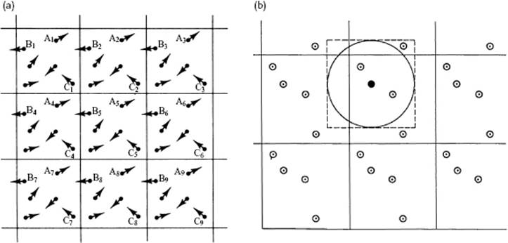
So let us now turn to the second aspect. To avoid having to calculate all interactions between all molecules, a cut-off value r_c for the individual interactions is used. In order for a particular interaction to contribute, the molecules should be within the cut-off distance: contributions of molecules further away are not taken into account. Of course, the cut-off value is arbitrary and is usually taken as the value where the interaction is less than, say, 10⁻⁴-fold the maximum interaction. It will be clear that the cut-off value determines the accuracy of the simulation. Typical values for the cut-off are 7 to 15 Å. Methods to correct (approximately) for the interactions outside this range exist; an example is the “tail” correction [1], which is used to calculate the potential energy contributions for r > r_c by assuming that the particles are uniformly distributed. In particular for long-range interactions, special techniques are required; an example for Coulomb interactions is the Ewald summation technique [2] which essentially makes clever use of lattice sums¹⁾ over the periodic images. The size of the meso-cell is typically chosen as at least double the cut-off value of the intermolecular interactions, so that a specific particle only interacts with the nearest image of the particles, keeping the book-keeping simple. In this way artifacts of periodicity are avoided, although care should be exercised: sudden cut-offs cause additional noise and erroneous behavior, while smooth cut-offs modify the interaction. For the cut-off volume using a cubic cell one can take either a cube (minimum image cut-off) or a sphere (spherical cut-off), as illustrated in Figure 9.1, leading to a slightly different number of interactions to be taken in to account. In order to avoid spurious non-isotropic interactions, nowadays almost always the spherical cut-off is often taken. The shape of the cell does influence the computational time, however, and choosing an optimal space-filling molecular-shaped cell that minimizes the volume while the distances between the atoms of images remain larger than a specified value is an option. Overall, the best strategy for homogeneous systems seems to be to use consistent potentials by including the complete lattice sums over the periodic images, but to combine this with a study of the behavior of the system as a function of cell size [2].

Within this framework one chooses the proper potential for the molecules and uses either the MD or MC method. Initially, the hard-sphere and Lennard-Jones potential were frequently chosen, and results of simulations with Lennard-Jones potentials are generally considered to be qualitatively reliable. Nowadays, more advanced empirical potentials containing many parameters are used. Such a potential is often called a force field. Preferably the force field should be transferable between different molecules and applicable to a wide range of conditions and environments. However, the non-additivity of constituent terms and the omission of contributions often renders these non-transferable. Since a force field usually contains adjustable parameters, a compensation of errors may occur and the optimum for one configuration under certain conditions is then not accurate for another condition under different conditions. A particularly clear discussion on force fields is provided by Berendsen [2].

The next two sections briefly introduce the MD and MC methods. The texts by Friedman [3] and Sachs et al. [4] also provide a short introduction to both methods, while Allen and Tildesley [5], Frenkel and Smit [6] and Berendsen [2] provide detailed discussions.