Liquid-State Physical Chemistry: Fundamentals, Modeling, and Applications (2013)
9. Modeling the Structure of Liquids: The Simulation Approach
9.3. The Monte Carlo Method
Whereas, in MD the structure and dynamics are calculated, in MC calculations attention is focused on the structure alone.
The method consists essentially of distributing molecules in space, calculating the associated energy, modifying the molecular distribution, and then repeating the calculation so as to obtain eventually a sequence of, say n, molecular distributions in configuration space that samples the desired ensemble (NVE, NVT, or otherwise) properly. If f represents any observable dependent only on the configuration, then each element of the sequence will generate a sample fj of the observable and the mean fm = n−1Σjfj is an estimator of the ensemble average ⟨f⟩. The essence of MC simulations is to construct the sequence in a smart fashion. The procedure is best explained by using ideas from calculating multidimensional integrals in numerical mathematics.
Suppose one has the integral
(9.16) ![]()
To evaluate this integral, the following trick is used. One writes
(9.17) ![]()
where f(x) > 0 over the interval [a,b] and f(x) is integrable. We treat f(x) as a probability density function so that ![]() . Then we can write
. Then we can write
(9.18) ![]()
where <h(x)> is the average value over the interval [a,b] assuming that x is distributed as f(x). Hence, it follows that if we choose points in the interval [a,b] at random5) with probability f(x) we can evaluate <h(x)> and by multiplying with the normalization factor F, calculate G.
In statistical thermodynamics we may wish to evaluate integrals such as
(9.19) ![]()
where the configurational partition function Q acts as a normalizing factor. Consequently, when we choose position vectors according to the distribution function
(9.20) ![]()
we can evaluate integrals of the type of Eq. (9.19). Unfortunately, Q, when acting as normalization factor, generally cannot be evaluated, but it is still possible to determine thermodynamic properties and structure.
The most frequently used method is that of Metropolis et al. [10], based on Markov processes. In this method one starts with an initial configuration of molecules and changes the configuration over a long sequence. The transition probabilities Tij of the transition from state6) i to state j are taken in such a way that in the infinite limit they tend to be distributed according to exp[−Φ(r1,…,rN)/kT]. Note that the total probability to end up in any state starting in state i is ΣjTij, so that we should have ΣjTij = 1. If ![]() is the probability to go from state i to state j in m steps, we have
is the probability to go from state i to state j in m steps, we have ![]() . It can be shown for Markov processes that, provided all states are accessible from any other state in a finite number of steps, the limit of
. It can be shown for Markov processes that, provided all states are accessible from any other state in a finite number of steps, the limit of ![]() for m → ∞ becomes Pj, independent of i. This implies that, after a sufficient number of steps, the state of the system is independent of the initial configuration. In the limit we have
for m → ∞ becomes Pj, independent of i. This implies that, after a sufficient number of steps, the state of the system is independent of the initial configuration. In the limit we have
(9.21) ![]()
stating that the probabilities are positive, that they are normalized, and that each state eventually is reached from any other state. We choose
(9.22) ![]()
From Eq. (9.22) it follows that we have the detailed balance condition
(9.23) ![]()
If we substitute this result in Eq. (9.21)–(9.23), we obtain the Pi = ΣjTjiPj = ΣjTijPi = PiΣjTij or ΣjTij = 1, satisfying our earlier requirement. Hence, by choosing the relationship between Tij and Tji according to Eq. (9.22), all requirements for a Markov process are fulfilled. What remains to be done is to choose the appropriate values for Tij.
Metropolis et al. used for Tij the following recipe
(9.24) 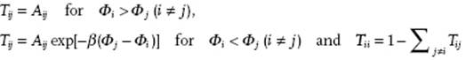
The constants Aij are chosen as Aij = Aji, and determined as follows:
· A molecule is chosen at random.
· A change in position (δx, δy, δz) is selected.
· Aij = 0 if any of |δx|, |δy| and |δz| > Δ, and Aij = (2Δ)−3 otherwise.
With these rules a large number of configurations is generated with the constant Δ chosen in such a way that about half of the configurations are accepted.
Calculations are initiated by providing the positions of N molecules in the cell chosen; this starting configuration can be selected as indicated in Section 9.1. Normally the first – say 200 000 – configurations are discarded in order to limit the influence of the starting configuration, and thereafter the properties are evaluated using, say 500 000, configurations. The above-outlined procedure is for the canonical ensemble, and enables one to calculate the ensemble average by direct sampling of phase space:
(9.25) ![]()
where Gj(r1, … ,rN) represents the value of G in configuration j. For example, the internal energy U is given by
(9.26) ![]()
where Ukin is the kinetic energy, given for spherical molecules by Ukin = 3NkT/2 and is due to the term Λ−3N. This can also be written as
(9.27) ![]()
so that the internal energy can be estimated by averaging the potential energy of all configurations in the MC sequence. The heat capacity is then
(9.28) ![]()
with CV,kin = 3Nk/2 the contribution of the kinetic energy to CV. The pressure can be calculated from the virial theorem expression (see Chapter 3) reading
(9.29) ![]()
with ∇i the gradient operator for molecule i. Finally, using the number of particles n(r) with distance between r and r + Δr from a reference particle and taking subsequently each particle as reference, from the expression
(9.30) ![]()
one can obtain the correlation function g(r).
Today, the MC method is used much like the MD method, more or less routinely, to calculate the properties of thermodynamic systems. Both, the MC and MD methods have the property of providing, in principle, exact calculations for a given interaction model, and the typical accuracy is about 1–2%. Provided that the same potentials are used and also the same conditions, the equilibrium results of the MD method agree to a large degree with those of the MC method (see Figure 9.3). Whereas, the MD method yields the full dynamics, it is somewhat more complex to eliminate time correlations when compared to the MC method.
Problem 9.3*
Is it possible to calculate QN in principle from a MC simulation?