Liquid-State Physical Chemistry: Fundamentals, Modeling, and Applications (2013)

10.4. Dielectric Behavior of Liquids

The question is now how well the approach as described before can be applied to liquids. Let us first consider mixtures of polar molecules in a nonpolar solvent. Figure 10.3 shows an example: C₆H₅NO₂ in hexane. We consider that the molar polarization of a mixture P_m is given by the rule of mixtures

where x_i is the mole fraction of the component i. The molar polarization P_i of each component i is, as before, given by

Figure 10.3 (a) Molar polarization P_m of the polar molecule C₆H₅NO₂ in the nonpolar solvent hexane as a function of mole fraction x (the small discontinuity at x ∼0.2 is due to the merging of two data sets); (b) The anomalous behavior of the molar polarization of water as function of inverse temperature.

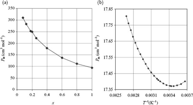
If the value for α_i for the nonpolar solvent is known, for example, using the refractive index, the value for μ_i of solute can be calculated given either the temperature-dependent data or independent data for α_i for the polar component. For the example mentioned we have μ = 3.9 D (α ≅ 0 C m² J⁻¹) as compared with μ = 4.2 D for the molecule in the gas phase. The agreement is good, which is true in general for molecules dissolved in nonpolar solvents. Because P_m is not necessarily linearly related to x_i, extrapolated values of P_m with x_i → 0 are often used, although in practice the permittivity of a mixture is often reasonably well described by a rule of mixtures using volume fractions for each component (but see Figure 10.3a).

The situation is quite different for pure liquids, however. For water, it is known that the dipole moment μ = 1.85 D and the polarizability volume α′ = 1.48 ų. If we calculate from these data the molar polarization via P_m = (α + μ²/3kT)N_A/3ε₀, and from that result the value of P_m/V_m, we obtain the value 4.2. Since P_m/V_m = (ε_r − 1)/(ε_r + 2) should be always smaller than 1, this result is physically impossible and such behavior is, therefore, occasionally called the “polarization catastrophe.” Moreover, it appears that the dielectric behavior of water (and other pure, polar liquids) is very unlike the Debye-behavior (Figure 10.3), due to shielding and correlation.

With regard to shielding, as indicated before, any molecule will experience a local field not equal to the applied field, because the surrounding molecules shield the applied field. In the Clausius–Mossotti and Debye models this effect was taken into account by using for both the internal and directional field the Lorentz internal field. However, it was argued that for the dipole contribution the directional field is different from the internal field, and taking this effect into account Onsager [4] derived an expression for the directional field. Although presenting all details of Onsager's calculations would lead us far astray, we nevertheless present an outline for a spherical molecule in a spherical cavity with radius a in Justification 10.1 (after all, this is beautiful physical chemistry!) from which we quote the result, preserving as much as possible the resemblance with the Debye equation,

(10.30)

Here, μ* = μ/(1 − fα) and α* = α/(1 − fα) with and 4πN_Aa³/3V_m = 1. This result implies, first, that the functional dependence on ε_r is changed and, second, that both the dipole moment μ* and polarizability α* in the condensed state are typically enhanced by 20–50% as compared to the gas state values μ and α by the near presence of other molecules. For example, for CHCl₃ with ε_r = 4.8 and n = 1.446 we obtain μ*/μ = 1.24 when using for α the Lorentz–Lorenz estimate . Introducing the expressions for f, a and α in Eq. (10.30), the explicit result for μ reads

(10.31)

which usually is denoted as the Onsager equation. From this equation, reasonable estimates of μ for nonassociating molecules can be obtained as compared to results from independent gas-phase experiments.

Now, on the subject of correlation, we assumed when calculating the average dipole moment that the alignment of the molecules was only due to the applied field. However, there is a correlation between neighboring molecules due to their mutual interaction, which results in a correction [5] for the value of (μ²/3kT) by a correlation factor g, defined via gμ² ≡ μ·μ* with μ* the dipole moment of the molecule and its immediate surroundings. More explicitly, the parameter g is determined by

(10.32)

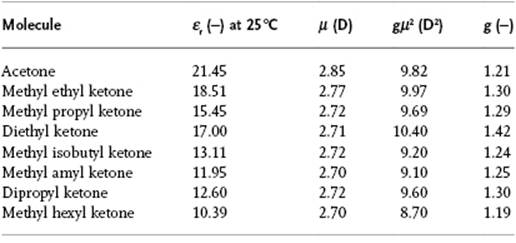
where N_j is the number of atoms in coordination shell j and ⟨cosγ_j⟩ the average cosine of the angle between the dipole of the (fixed) reference molecule and the molecules in shell j. The molecular dipoles tend to line up, but are counteracted by geometric packing effects. If the dipole moment is along the long axis of the molecule, close packing forces more molecules to have γ ≅ 90° and g < 1. In case the dipole moment is along the short axis of the molecule, packing effects result in having more molecules with γ ≅ 0° and g > 1. The correlation function, however, cannot be determined experimentally in an independent way, and accurate information on structure and intermolecular interactions is required for its calculation. It should be noted from the data in Table 10.6 that there is neither correlation between g and ε, nor between g and μ. One would expect, however, that in a series of similar molecules using independent values for the dipole moments similar values for g are obtained. Table 10.7 shows that, for aliphatic ketones, this is indeed the case. Unfortunately, however, the theoretical treatment of the Kirkwood factor is involved and we have to refer to the literature.⁶⁾

Table 10.6 Estimates of Kirkwood's correlation factor g for several polar molecules.^a)

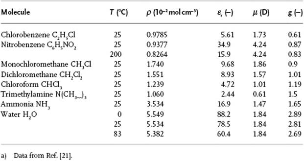
Table 10.7 Values of g for aliphatic ketones [2].

One factor not taken into account in the previous analysis was the associa­tion of molecules, in particular via hydrogen bonding. This effect is particularly important for water. If the Kirkwood model is applied to water at 0 °C using a model where every molecule is hydrogen-bonded to four neighbors and taking into account interactions up to the 4th shell, using N₁ = 4, N₂ = 11, N₃ = 22, the contributions g₁, g₂ and g₃ of the first, second and third shells to g are 1.20, 0.33 and 0.07, respectively, and a g-value of ∼2.6 is obtained. It appears therefore that correlation with shells outside the first shell results in an appreciable contribution to the total dielectric polarization. The permittivity obtained is ε_r = 71.9, which is in reasonable agreement with the experimental value ε_r = 88.0 [6], while the dipole moment was estimated as μ* = 2.17 D, some 17% larger than for the gas state, μ = 1.85 D. For ice [7] at 0 °C, Coulson and Eisenberg calculated μ* = 2.60 D, which was some 40% larger than μ = 1.85 D. Whilst for water a reasonable agreement is obtained using the Kirkwood model, for aliphatic alcohols the values obtained are close to those as calculated from the Onsager model, and differ considerably from the experimental data. For further details we refer to the literature⁶⁾.

Justification 10.1: The internal, reaction, and directional field*

In this justification an outline of the Onsager calculation is given. For full details we refer to Böttcher [1]. We first quote some results from electrostatics, of which a brief discussion is given in Appendix D, and thereafter describe the internal, reaction, and directional fields leading to the Clausius–Mossotti, Debye, and Onsager equations using the abbreviation .

From electrostatics (see Appendix D) we borrow the expression for the field E_cav inside a spherical cavity with radius a, embedded in a dielectric with relative permittivity ε_r and provided with an external field E, reading

(10.33)

If a nonpolarizable spherical molecule with dipole moment μ is placed in the center of such a cavity without any applied field E, the molecule polarizes the dielectric and this polarization in turn creates a reaction field R on the molecule. The reaction field R appears to be uniform, is proportional to the dipole moment μ, and given by R = f μ with . If the molecule is polarizable with polarizability α, the reaction field is due to the permanent dipole μ and the induced dipole αR, so that we have R = f(μ + αR). Solving for R, we obtain

(10.34)

Now, recall that in the case where a field E is applied, the dielectric displacement D = ε₀ε_rE = ε₀E + P with polarization P = ε₀(ε_r − 1)E. The total polarization is thought to be composed of the polarization P_μ due to the dipole μ of the molecules, and the polarization P_α due to the polarizability αof the molecules. We assume that P_α equals the product ραE_int with E_int = E_cav + R the internal field, and ρ = N/V the number density of the polarizable molecules. For P_μ we have with the rotational average of μ. Onsager argued that for P_μ only the directional field E_dir, defined as with the rotational average of R, is active. So, generally

(10.35)

where the Langevin estimate for is used.

Let us focus first on nonpolar but polarizable molecules. The conventional approach to estimating the internal field is due to Lorentz, who assumed that the reference molecule is surrounded by an imaginary sphere of such a size that the material outside the sphere could be treated as a continuum. If the reference molecule is removed, then the total field in the sphere would be due to the applied field E, the field E_sphere due to free ends of the surrounding dipoles covering the sphere, and the field E_mol due to molecules in the near-vicinity of the reference molecule. The latter field averages to zero for a sufficiently high symmetry. The component of E_sphere in the direction of E is calculated by integrating the field of infinitesimal rings perpendicular to the field direction. The apparent surface charge density on these rings is Pcosθ, while their surface is 2πr²sinθ dθ, leading to a total charge on each ring of dq = 2πr²Psinθ cosθ dθ. According to Coulomb's law, each charge element contributes to the field by . Combining yields . Due to symmetry, the other contributions vanish so that E_int becomes E_int = E + P/3 = E(ε_r + 2)/3. Introducing E_int in P_α = (ραE_int) = ε₀(ε_r − 1)E yields

(10.36)

known as the Clausius–Mossotti equation. An alternative derivation due to Onsager uses the cavity field E_cav = 3ε_rE/(2ε_r + 1), and the reaction field R. The latter is in this case R = f (αE_cav + αR). Solving for R leads to

(10.37)

Because E_int = E_cav + R, the result is

(10.38)

Onsager further assumed that the relationship 4πρa³/3 = 1 holds. Putting this together with the expression for f, one obtains from Eq. (10.35) with P_μ = 0 (after some manipulation) again the Clausius–Mossotti equation. This alternative derivation makes the assumption on the cavity size clear.

We now turn to polar polarizable molecules. Debye used the Lorentz internal field E_int = E(ε_r + 2)/3 for both P_μ and P_α in Eq. (10.35), and this in turn leads to the Debye equation

(10.39)

Onsager used E_dir and to calculate E_int and obtained

(10.40)

(10.41)

The internal field E_int is obtained from resulting in

(10.42)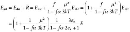

Finally, substituting E_dir and E_int, together with the expression for f, in Eq. (10.35) leads, after considerable manipulation, to the Onsager equation

(10.43)

Further substitution of the expression for f, the condition 4πρa³/3 = 1 and the Lorentz–Lorenz estimate and explicitly solving for μ leads to Eq. (10.31). Further refinements include the use of an ellipsoidal rather than a spherical cavity, the use of an ellipsoidal rather than a spherical molecule, and the use of a fixed cavity size for the Clausius–Mossotti equation [1]. These refinements all improve the agreement of the value for μ with results of independent experiments.

Problem 10.10

For methanol (T_m = −98 °C, ρ = 0.791 g cm⁻³ at 20 °C), ε_r data corrected for density are given below. Determine α and μ for methanol.

What further information can be retrieved from these data?

Problem 10.11

Calculate μ*/μ for propanone with ε_r = 21.4 and n = 1.359.

Problem 10.12

For C₂H₅Br (ρ = 1.43 g cm⁻³), μ = 6.67 × 10⁻³⁰ C m, and α = 11.1 × 10⁻⁴⁰ C m² V⁻¹.

a. Calculate ε_r for this liquid, using the Debye equation and Onsager equation.

b. Comment on the agreement of the results of a) and b) with the experimental value ε_r = 9.3.