Liquid-State Physical Chemistry: Fundamentals, Modeling, and Applications (2013)
11. Mixing Liquids: Molecular Solutions
So far, we have discussed pure liquids with increasing complexity. In this chapter we start with solutions and, in particular, with molecular solutions. We first deal briefly with some basic aspects, including molar and partial quantities, perfect, and ideal solutions. Thereafter, nonideal behavior is discussed, based on a treatment of the regular solution model. Finally, some possible improvements are indicated.
11.1. Basic Aspects
In this section we iterate and extend somewhat on some of the basic aspects that were introduced in Chapter 2. The content of a system is defined by the amount of moles nα of chemical species α in the system, often denoted as components, which can be varied independently. A mixture is a system with more than one component. A homogeneous part of a mixture, that is, with uniform properties, is addressed as a phase, while a multicomponent phase is labeled a solution. The majority component of a solution is the solvent, while solute refers to the minority component. We restrict ourselves from the outset to binary mixtures and solutions and use, apart from nα for the number of moles, Nα for the number of molecules and xα for the mole fraction of component α. The label 1 refers always to the solvent (e.g., x1 or 1 − x), while the label 2 indicates the solute (e.g., x2 or x). As usual, NA denotes Avogadro's constant.
11.1.1 Partial and Molar Quantities
We refer for an arbitrary extensive quantity Z of a mixture to molar quantities Zm defined by Zm = Z/Σαnα or for single, pure component α by ![]() . For solutions, it is also useful to discuss the situation with respect to extensive quantities Z in terms of partial (molar) quantities Zα ≡ (∂Z/∂nα)P,T,n′, where n′ indicates all components except for the component α. Generally, for Z = Z(P,T,nα), we have
. For solutions, it is also useful to discuss the situation with respect to extensive quantities Z in terms of partial (molar) quantities Zα ≡ (∂Z/∂nα)P,T,n′, where n′ indicates all components except for the component α. Generally, for Z = Z(P,T,nα), we have
(11.1) ![]()
Since the extensive quantity Z(P,T,nα) is a homogeneous function of degree 1 in nα, we have by Euler's theorem1)
(11.2) ![]()
So, we have for dZ on the one hand Eq. (11.1), and on the other hand differentiating Eq. (11.2) dZ = ΣαZαdnα + ΣαnαdZα. Hence,
(11.3) 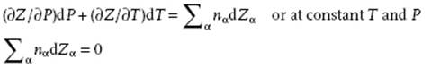
This is the (general) Gibbs–Duhem equation, which puts a constraint on the possible changes in the properties of solutions.
For the volume, the partial volume is given by Vα = (∂V/∂nα)P,T,n′ and the total volume becomes at constant T and P, using Euler's theorem,
(11.4) ![]()
Similarly, for the Gibbs energy G we have the partial Gibbs energy Gα = (∂G/∂nα)P,T,n′, and since this quantity is equal to the chemical potential defined by μα ≡ (∂G/∂nα)P,T,n′, the total Gibbs energy becomes
(11.5) ![]()
Note that the partial quantity Gα and chemical potential μα are equivalent, but that for the Helmholtz energy F one would have μα = (∂F/∂nα)V,T,n′ ≠(∂F/∂nα)P,T,n′ = Fα.
For the Gibbs energy G we further obtain at constant P and T
(11.6) ![]()
This is the Gibbs–Duhem equation (at constant P and T) of which another form is
(11.7) ![]()
where ![]() is the chemical potential of the pure component 1. This relation can be used for a consistency check on experimental data. If the molar Gibbs energy Gm is known, we can obtain μ1 and μ2 by differentiation with respect to x2, since
is the chemical potential of the pure component 1. This relation can be used for a consistency check on experimental data. If the molar Gibbs energy Gm is known, we can obtain μ1 and μ2 by differentiation with respect to x2, since
(11.8) ![]()
and solving μ1 and μ2 from Eq. (11.5) and (11.8) results in
(11.9) 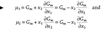
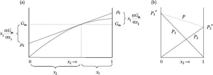
Thus, if the dependence of Gm as function of x2 (or x1 for that matter) is known (Figure 11.1), the behavior of μ1 and μ2 can be obtained by differentiation. It will be clear that a similar reasoning applies to all partial quantities, for example, Vm. It will also be evident that Gm is less easily accessible experimentally than Vm.
Figure 11.1 (a) Calculation of the chemical potentials μ1 and μ2 from the Gibbs energy Gm (although illustrated here for μ1 and μ2 using Gm, this calculation can be made for any partial quantity, remembering that μα equals Gα); (b) Pressure diagram for a perfect mixture, showing the total pressure P and the partial pressures P1 and P2.
11.1.2 Perfect Solutions
To describe perfect solutions we start with the perfect gas, and thereafter deal with perfect gas mixtures and generalize to perfect (fluid) mixtures. The perfect gas can be defined in several ways. Here, we choose a definition based on the chemical potential
(11.10) ![]()
where P is the pressure, P° is a reference pressure (1 bar), and μ° is the value for μ = Gm = G/n if P = P°. From this definition we obtain for an arbitrary number of moles n, V = ∂G/∂P = ∂(nμ)/∂P = nRT/P, the well-known equation of state (EoS) for a perfect gas. Hence
(11.11) ![]()
For perfect gas mixtures we assume that each component contributes independently from the others to the Helmholtz energy, so that we have
(11.12) ![]()
This leads to
(11.13) ![]()
where Pα ≡ xαP is referred to as the partial pressure2). The total pressure is accordingly given by P = ΣαPα or, for a perfect binary mixture, by (Figure 11.2)
(11.14) ![]()
known as Dalton's law of partial pressures. For the perfect gas mixture the partial volume becomes Vα = ∂μα/∂P = ∂ lnPα/∂P = RT/P, equal for all components α.
To calculate ΔmixG for a binary gas mixture at ![]() and
and ![]() we subtract n1μ1 + n2μ2 at P1′ and P2′ from Gmix to obtain
we subtract n1μ1 + n2μ2 at P1′ and P2′ from Gmix to obtain
(11.15) 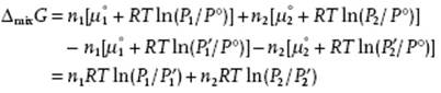
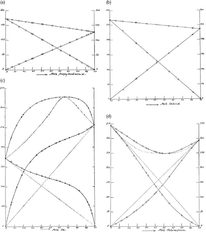
Figure 11.2 The vapor pressure of the ideally behaving system for: (a) Propylene bromide/ethylene bromide at 85 °C; (b) Ethylene chloride/benzene at 50 °C; (c) Positively-deviating-from-ideality system carbon disulfide/acetone at 35 °C; (d) Negatively-deviating-from-ideality system chloroform/acetone at 35 °C. Many books have used von Zawidski's data [20], usually without reference. It is therefore appropriate to show some of his original figures.
From this expression we obtain the entropy of mixture ΔmixS as
(11.16) 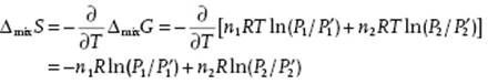
In the special case that ![]() , that is, when the original pressures of each gas
, that is, when the original pressures of each gas ![]() and
and ![]() are equal to the final pressure P′, we have
are equal to the final pressure P′, we have ![]() and
and
(11.17) ![]()
A perfect solution is defined as having the same Gibbs energy of mixing as the perfect gas mixture for the whole composition range, that is, for one mole
(11.18) ![]()
Equivalently, we have
(11.19) ![]()
Equation (11.19) forms the basis for all further treatments. In practice only very few systems behave as a perfect mixture, and perfect behavior usually involves a comparable chemical nature of the solvent and solute, although this provides neither a guarantee, nor is required. Generally, strong deviations are observed. An example of both types of near-perfect solutions is shown in Figure 11.2, as are examples of a negative and positive from ideal behavior-behaving systems.
Problem 11.1
Recall that a real gas can be described by the virial expansion
![]()
Using the inversion of the virial expansion in terms of P, show that the expression for G becomes
![]()
leading for sufficient low pressure to μ = μ° + RT ln (P/P°).
Problem 11.2
Show that for a perfect gas the energy U depends only on the temperature T.
Problem 11.3
Show that for a perfect gas mixture, ΔmixH and ΔmixV are both identically zero.
Problem 11.4
Verify Eq. (11.9).
Problem 11.5
Suppose that the molar volume of a binary solution of components 1 and 2 is given by ![]() . Calculate the partial volumes V1 and V2.
. Calculate the partial volumes V1 and V2.
Problem 11.6
Suppose that the partial volume of solute 2 in solvent 1 is given by V2 = a + b(1 − x2)2, while the molar volume Vm (1) of the pure solvent is given by c. Calculate the partial molar volume V1 using the Gibbs–Duhem equation.