Liquid-State Physical Chemistry: Fundamentals, Modeling, and Applications (2013)

11.2. Ideal and Real Solutions

Perfect solutions behave as perfect gas mixtures over the complete concentration range. In practice, perfect solution behavior is obeyed only for a limited range of concentrations, and we label these cases as ideal solutions. For perfect and ideal behavior, a number of consequences follow of which we describe Raoult's and Henry's laws. Thereafter, we discuss how to deal with real solutions.

11.2.1 Raoult's and Henry's Laws

For ideal solutions we have (within the range of validity) the expression

(11.20)

while for the perfect gas the expression

(11.21)

holds. Using the equilibrium condition μ(sol) = μ(vap), we easily obtain

(11.22)

Solving for P_α leads to

(11.23)

The parameter K_H,α is independent of composition. For the solute we have

(11.24)

known as Henry's law (1803!), and stating that the partial pressure P₂ of solute 2 is proportional to the mole fraction in the liquid phase with a proportionality constant dependent on the difference in chemical potential, that is, in interaction, between solvent 1 and solute 2. For the solvent, the limiting situation is x₁ = 1 for which . Hence approximately

(11.25)

known as Raoult's law (1886–1887), and stating that the partial pressure P₁ of solvent 1 is directly proportional to the vapor pressure of the pure solvent. Obviously, for perfect solutions Raoult's law is valid for the complete composition range.

Some data for Henry's constant are given in Table 11.1. Example 11.1 shows how to use these concepts.

Table 11.1 Henry's constant K_H for gases dissolved in H₂O and C₆H₆ (in brackets) at 25 °C.^a)

a) Data from Refs [21, 22].

Example 11.1

Assuming that sparkling water contains only H₂O (1) and CO₂ (2), we want to determine for a sealed can the compositions of the vapor and liquid phases and the pressure exerted at 10 °C, knowing that Henry's constant for CO₂ in H₂O at 10 °C is about 990 bar. There is only one degree of freedom according to the phase rule. We use the mole fraction x₂ of CO₂ in the liquid and assume it is 0.01. We denote the mole fraction in the gas phase by y. For the solute (2) we have Henry's law, while for the solvent (1) Raoult's law applies.

With K_H,2 = 990 bar and (steam tables at 10 °C or Antoine's equation), P = 9.912 bar. By Raoult's law, . Therefore, y₂ = 1 − y₁ = 0.9988. As expected, the vapor is nearly pure CO₂.

11.2.2 Deviations

To describe deviations from perfect solution behavior we have a few options. The most well-known option is introducing the activity a = γ x, where γ is the activity coefficient. The activity coefficient γ_α = γ_α(T,x) is introduced “to keep up appearances,” that is, to keep the same formal expression for μ_α as for the perfect solution. Hence, becomes , with activity a_α = γ_αx_α. Obviously, γ_ideal = 1 always. There are two conventions for the activity coefficient.

· Convention I: γ_α → 1 for x_α → 1 and for x_α → 0. This convention is usually employed if the (liquid) solute is fully soluble in the solvent. Because, in a dilute solution of component β in α, molecules of type α are mainly surrounded by molecules of type α, component α behaves largely as if the liquid was pure. The reference state is thus the chemical potential of the pure liquid . This convention is also referred to as Raoult's law convention.

· Convention II: γ₁ → 1 for x₁ → 1 and γ₂ → 1 for x₂ → 0. This convention is usually employed if the (solid or liquid) solute is only partially soluble in the solvent. For the solvent this convention is identical to convention I. Because, in a dilute solution of component 2 in 1, molecules of type 2 do not interact with each other but mainly with molecules of type 1, the activity coefficient approaches a constant value, characteristic for the 1–2 interaction. Since we would like to have γ₂ → 1 for x₂ → 0, the reference state for the solute is taken as that of the pure solute in a hypothetical liquid state extrapolated to infinite dilution using Henry's law. Accordingly, this convention is referred to as Henry's law convention.

From the Gibbs–Duhem equation x₁dμ₁ + x₂dμ₂ = 0, we obtain (using μ = μ* + RT lnγ x) x₁ d lnγ₁ + x₂ d lnγ₂ = 0. Similarly, as for Eq. (11.7), some manipulation results in

(11.26)

where γ_1,0 is the limiting value of γ₁ for x₁ → 0. Since for x₁ → 0, γ₁ → 1, the lower limit in the second integral should be taken as zero. This relation provides a check on the experimental data for γ₁ and γ₂ or allows one to calculate γ₂ if γ₁ is known.

Another way to introduce deviations from ideal behavior is by introducing the osmotic coefficients g and ϕ, defined for the solvent by

(11.27)

where the molality m₂ = x₂/x₁M₁ and the mole fraction x₁ = (1 + m₂M₁)⁻¹ are used (why g and ϕ are addressed as osmotic coefficients will become clear in the next section). Since for high dilution we should regain ideal behavior, we require that for x₁ → 1, g → 1, and thus ϕ → 1. We have the relations lnγ₁ = (g − 1)lnx₁ and ϕ = −(m₂M₁)⁻¹g ln (1 + m₂M₁)⁻¹ ≅ g (1 − ½m₂M₁ + …).

We also can define excess functions by

(11.28)

The partial quantities Z_α are directly related to the excess quantities Z^E. For example, for G we have Z_α = G_α = μ_α and substitution of Eq. (11.7) in , dividing by x₁ = 1 − x₂ and differentiating with respect to x₂ yields

(11.29)

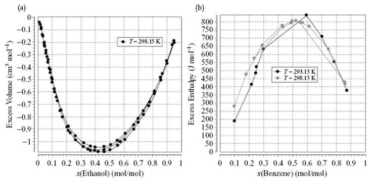
It is a matter of convenience whether excess or partial quantities are used. Figure 11.3 shows two examples of excess functions.

Figure 11.3 (a) Excess volume V^E for a mixture of H₂O–C₂H₅OH; (b) Excess enthalpy H^E for a mixture of benzene in cyclohexane. Images obtained from the Dortmund Data Base.

Problem 11.7

Verify Eq. (11.26) and (11.27).